Page 18 - Statistics for Environmental Engineers

L1592_Frame_C02 Page 9 Tuesday, December 18, 2001 1:40 PM

The ordinate of the histogram can be the actual count (n i ) of occurrences in an interval or it can be
the relative frequency, f i = n i /n, where n is the total number of values used to construct the histogram.
Relative frequency provides an estimate of the probability that an observation will fall within a particular
interval.
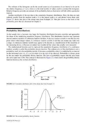
Another useful plot of the raw data is the cumulative frequency distribution. Here, the data are rank
ordered, usually from the smallest (rank = 1) to the largest (rank = n), and plotted versus their rank.
Figure 2.3 shows this plot of the nitrate data from Example 2.1. This plot serves as the basis of the
probability plots that are discussed in Chapter 5.

Probability Distributions

As the sample size, n, becomes very large, the frequency distribution becomes smoother and approaches
the shape of the underlying population frequency distribution. This distribution function may represent
discrete random variables or continuous random variables. A discrete random variable is one that has only
point values (often integer values). A continuous random variable is one that can assume any value over
a range. A continuous random variable may appear to be discrete as a manifestation of the sensitivity of
the measuring device, or because an analyst has rounded off the values that actually were measured.
The mathematical function used to represent the population frequency distribution of a continuous
random variable is called the probability density function. The ordinate p(y) of the distribution is not a
probability itself; it is the probability density. It becomes a probability when it is multiplied by an interval
on the horizontal axis (i.e., P = p(y)∆ where ∆ is the size of the interval). Probability is always given
by the area under the probability density function. The laws of probability require that the area under
the curve equal one (1.00). This concept is illustrated by Figure 2.4, which shows the probability density
function known as the normal distribution.

12
Nitrate (mg/L) 8

4
0 10 20 30
Rank Order

FIGURE 2.3 Cumulative distribution plot of the nitrate data from Example 2.1.

0.4
Probability Density, p(y) 0.3 Area =

P = p( y) ∆
0.2

0.1

0.0 ∆ y
-4 -3 -2 -1 0 1 2 3 4

FIGURE 2.4 The normal probability density function.

© 2002 By CRC Press LLC