Page 208 - Statistics for Environmental Engineers

l1592_frame_Ch23 Page 208 Tuesday, December 18, 2001 2:44 PM

Example 23.8

∗
We expect the control survival proportion to be p c = 0.95 and we wish to detect effluent toxicity
∗
corresponding to an effluent survival proportion of p e = 0.75. The probability of detecting a real
effect is to be 1 − β = 0.9 (β = 0.1) with confidence level α = 0.05. The transformed proportions
are x c = arcsin 0.95 = 1.345 and x e = arcsin 0.8 = 1.047, giving δ = 1.345 − 1.047 = 0.298.
Using z 0.05 = 1.645 and z 0.1 = 1.282 gives:
1.645 +

1.282
n = 0.5 ---------------------------------  2 = 48.2
 1.345 1.047
–
This would probably be adjusted to n = 50 organisms for each test condition.
This may be surprisingly large although the design conditions seem reasonable. If so, it may
indicate an unrealistic degree of confidence in the widely used design of n = 20 organisms. The
number of organisms can be decreased by increasing α or β, or by decreasing δ.

This approach has been used by Cohen (1969) and Mowery et al. (1985). An alternate approach is given
by Fleiss (1981). Two important conclusions are (1) there is great statistical benefit in having the control
proportion high (this is also important in terms of biological validity), and (2) small sample sizes (n < 20)
are useful only for detecting very large differences.

Stratified Sampling
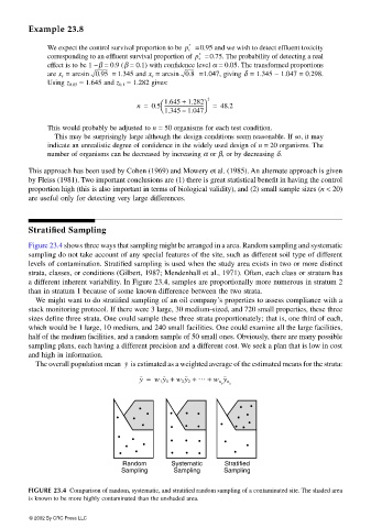
Figure 23.4 shows three ways that sampling might be arranged in a area. Random sampling and systematic
sampling do not take account of any special features of the site, such as different soil type of different
levels of contamination. Stratified sampling is used when the study area exists in two or more distinct
strata, classes, or conditions (Gilbert, 1987; Mendenhall et al., 1971). Often, each class or stratum has
a different inherent variability. In Figure 23.4, samples are proportionally more numerous in stratum 2
than in stratum 1 because of some known difference between the two strata.
We might want to do stratified sampling of an oil company’s properties to assess compliance with a
stack monitoring protocol. If there were 3 large, 30 medium-sized, and 720 small properties, these three
sizes define three strata. One could sample these three strata proportionately; that is, one third of each,
which would be 1 large, 10 medium, and 240 small facilities. One could examine all the large facilities,
half of the medium facilities, and a random sample of 50 small ones. Obviously, there are many possible
sampling plans, each having a different precision and a different cost. We seek a plan that is low in cost
and high in information.
The overall population mean is estimated as a weighted average of the estimated means for the strata:
y
y = w 1 y 1 + w 2 y 2 + … + w n s y n s

• •
•
• • • • •
• • •
• •
•
• • • • •
•
•
• • • •
•
• •
• •
• • • •
Random Systematic Stratified
Sampling Sampling Sampling
FIGURE 23.4 Comparison of random, systematic, and stratified random sampling of a contaminated site. The shaded area
is known to be more highly contaminated than the unshaded area.
© 2002 By CRC Press LLC