Page 204 - Statistics for Environmental Engineers

l1592_frame_Ch23 Page 204 Tuesday, December 18, 2001 2:44 PM

Stein and Dogansky (1999) give an iterative solution for the case where a different sample size will
be taken for each treatment. This is desirable when data from the standard process is already available.
In the interval hypothesis, the type I error rate (α) denotes the probability of falsely declaring
equivalence. It is often set to α = 0.05. The power of the hypothesis test (1 − β ) is the probability of
correctly declaring equivalence. Note that the type I and type II errors have the reverse interpretation
from the classical hypothesis formulation.

Example 23.5

A standard process is to be compared with a new process. The comparison will be based on
taking a sample of size n from each process. We will consider the two process means equivalent
if they differ by no more than 3 units (θ = 3.0), and we wish to determine this with risk levels
α = 0.05, β = 0.10, σ = 1.8, when the true difference is at most 1 unit (∆ = 1.0). The sample
size from each process is to be equal. For these conditions, z 0.05 = 1.645 and z 0.10 = 1.28, and:

(
2 1.8) 1.645 +( 1.28) 2
2
n = ------------------------------------------------------- + 1 ≈ 15
( 3.0 1.0) 2
–

Confidence Interval for an Interaction

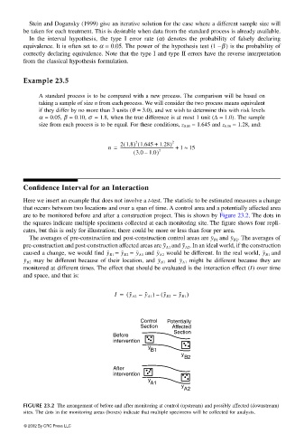
Here we insert an example that does not involve a t-test. The statistic to be estimated measures a change
that occurs between two locations and over a span of time. A control area and a potentially affected area
are to be monitored before and after a construction project. This is shown by Figure 23.2. The dots in
the squares indicate multiple specimens collected at each monitoring site. The figure shows four repli-
cates, but this is only for illustration; there could be more or less than four per area.
. The averages of
The averages of pre-construction and post-construction control areas are y B1 and y B2
. In an ideal world, if the construction
pre-construction and post-construction affected areas are y A1 and y A2
and
caused a change, we would find y B1 = y B2 = y A1 and y A2 would be different. In the real world, y B1
might be different because they are
y B2 may be different because of their location, and y B1 and y A1
monitored at different times. The effect that should be evaluated is the interaction effect (I) over time
and space, and that is:
I = ( y A2 – y A1 ) ( y B2 – y B1 )
–

Control Potentially
Section Affected
Section
Before • •
intervention • • • •
y • •
B1
y
B2
After • •
intervention • • • •
y • •
A1
y
A2
FIGURE 23.2 The arrangement of before and after monitoring at control (upstream) and possibly affected (downstream)
sites. The dots in the monitoring areas (boxes) indicate that multiple specimens will be collected for analysis.
© 2002 By CRC Press LLC