Page 201 - Statistics for Environmental Engineers

l1592_frame_Ch23 Page 201 Tuesday, December 18, 2001 2:44 PM

If this condition is satisfied, the confidence interval for η 1 − η 2 does not include zero and we do
not reject the hypothesis that the true change could be as large as 25 units.
The standard error of the difference is:

1
1
s y −y = s pool ---- + ----
1 2
n 1 n 2
which is estimated with ν = n 1 + n 2 − 2 degrees of freedom. Assuming the variances before and
after the intervention are the same, s 1 = s 2 = 58 and therefore s pool = 58.
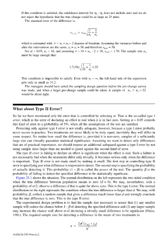
For α = 0.05, n 1 = 10, and assuming ν = 10 + n 2 − 2 > 30, t 0.05 = 1.70. The sample size n 2
must be large enough that:

1
1
(
1.7 58) ------ + ---- ≤ 25
10 n 2
This condition is impossible to satisfy. Even with n 2 = ∞, the left-hand side of the expression
gets only as small as 31.2.
The managers should have asked the sampling design question before the pre-change survey
was made, and when a larger pre-change sample could be taken. A sample of n 1 = n 2 ≈ 32
would be about right.

What about Type II Error?

So far we have mentioned only the error that is controlled by selecting α. That is the so-called type I
error, which is the error of declaring an effect is real when it is in fact zero. Setting α = 0.05 controls
this kind of error to a probability of 5%, when all the assumptions of the test are satisfied.
Protecting only against type I error is not totally adequate, however, because a type I error probably
never occurs in practice. Two treatments are never likely to be truly equal; inevitably they will differ in
some respect. No matter how small the difference is, provided it is non-zero, samples of a sufficiently
large size can virtually guarantee statistical significance. Assuming we want to detect only differences
that are of practical importance, we should impose an additional safeguard against a type I error by not
using sample sizes larger than are needed to guard against the second kind of error.
The type II error is failing to declare an effect is significant when the effect is real. Such a failure is
not necessarily bad when the treatments differ only trivially. It becomes serious only when the difference
is important. Type II error is not made small by making α small. The first step in controlling type II
error is specifying just what difference is important to detect. The second step is specifying the probability
of actually detecting it. This probability (1 – β) is called the power of the test. The quantity β is the
probability of failing to detect the specified difference to be statistically significant.
Figure 23.1 shows the situation. The normal distribution on the left represents the two-sided condition
when the true difference between population means is zero (δ = 0). We may, nevertheless, with a
probability of α/2, observe a difference d that is quite far above zero. This is the type I error. The normal
distribution on the right represents the condition where the true difference is larger than d. We may, with
probability β, collect a random sample that gives a difference much lower than d and wrongly conclude
that the true difference is zero. This is the type II error.
The experimental design problem is to find the sample size necessary to assure that (1) any smaller
sample will reduce the chance below 1– β of detecting the specified difference and (2) any larger sample
may increase the chance well above α of declaring a trivially small difference to be significant (Fleiss,
1981). The required sample size for detecting a difference in the mean of two treatments is:

2
2σ z α/2 +( z β )
n = ---------------------------------
∆ 2
© 2002 By CRC Press LLC