Page 200 - Statistics for Environmental Engineers

l1592_frame_Ch23 Page 200 Tuesday, December 18, 2001 2:44 PM

deviation is s = 58.0. The 95% confidence interval of this estimate is calculated using t 9,0.025 = 2.228:
s
58.0
y ± t 9,0.025 ------- = 234.2 ± 2.228---------- = 234.2 ± 40.8
n 10
The true mean lies in the interval 193 to 275.
What sample size is needed to estimate the true mean with ±20 units? Assume the needed
sample size will be large and use z = 1.96. The solution is:
(
n =   z α /2 σ  2 =   1.96 58)   2 = 32
------------
---------------------
E 
20
Ten of the recommended 32 observations have been made, so 22 more are needed. The recom-
mended sample size is based on anticipation of σ = 58. The σ value actually realized may be
more or less than 58, so n = 32 observations may give an estimation error more or less than the
target of ±20 units.
The approximation using z = 2.0 leads to n = 34.

The number of samples in Example 23.2 might be adjusted to obtain balance in the experimental design.
Suppose that a study period of about 4 to 6 weeks is desirable. Taking n = 32 and collecting specimens
on 32 consecutive days would mean that four days of the week are sampled five times and the other
three days are sampled four times. Sampling for 35 days (or perhaps 28 days) would be a more attractive
design because each day of the week would be sampled five times (or four times).
In Examples 23.1 and 23.2, σ was estimated by calculating the standard deviation from prior data.
Another approach is to estimate σ from the range of the data. If the data come from a normal distribution,
the standard deviation can be estimated as a multiple of the range. If n > 15, the factor is 0.25 (estimated
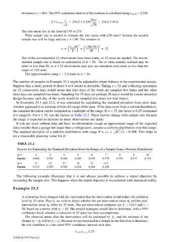
σ = range/4). For n < 15, use the factors in Table 23.2. These factors change with sample size because
the range is expected to increase as more observations are made.
If you are stuck without data and have no information except an approximate range of the expected
data (smaller than a garage but larger than a refrigerator), assume a uniform distribution over this range.
The standard deviation of a uniform distribution with range R is s U = R /12 = 0.29R. This helps to
2
set a reasonable planning value for σ.
TABLE 23.2
Factors for Estimating the Standard Deviation from the Range of a Sample from a Normal Distribution
n == == 2 3 4 5 6 7 8 9 10
Factor 0.886 0.591 0.486 0.430 0.395 0.370 0.351 0.337 0.325
n == == 11 12 13 14 15 >15
Factor 0.315 0.307 0.300 0.294 0.288 0.250

The following example illustrates that it is not always possible to achieve a stated objective by
increasing the sample size. This happens when the stated objective is inconsistent with statistical reality.
Example 23.3

A system has been changed with the expectation that the intervention would reduce the pollution
level by 25 units. That is, we wish to detect whether the pre-intervention mean η 1 and the post-
intervention mean η 2 differ by 25 units. The pre-intervention estimates are = 234.3 and s 1 =y 1
58, based on a survey with n 1 = 10. The project managers would like to determine, with a 95%
confidence level, whether a reduction of 25 units has been accomplished.
and the estimate of the
The observed mean after the intervention will be estimated by y 2
– will be y 1 – . Because we are interested in a change in one direction (a decrease),
change η 1 η 2 y 2
the test condition is a one-sided 95% confidence interval such that:
t ν,0.05 s y −y ≤ 25
1 2
© 2002 By CRC Press LLC