Page 199 - Statistics for Environmental Engineers

l1592_frame_Ch23 Page 199 Tuesday, December 18, 2001 2:44 PM

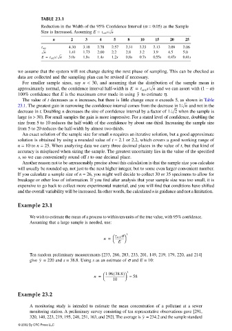
TABLE 23.1
Reduction in the Width of the 95% Confidence Interval (α = 0.05) as the Sample
Size is Increased, Assuming E = t α/2 s/ n
n 2 3 4 5 8 10 15 20 25
4.30 3.18 2.78 2.57 2.31 2.23 2.13 2.09 2.06
t α/2
n 1.41 1.73 2.00 2.2 2.8 3.2 3.9 4.5 5.0
E = t α/2 s/ n 3.0s 1.8s 1.4s 1.2s 0.8s 0.7s 0.55s 0.47s 0.41s

we assume that the system will not change during the next phase of sampling. This can be checked as
data are collected and the sampling plan can be revised if necessary.
For smaller sample sizes, say n < 30, and assuming that the distribution of the sample mean is
approximately normal, the confidence interval half-width is E = t α/2 s/ n and we can assert with (1 – α)
100% confidence that E is the maximum error made in using to estimate η.y
The value of t decreases as n increases, but there is little change once n exceeds 5, as shown in Table
23.1. The greatest gain in narrowing the confidence interval comes from the decrease in 1/ n and not in the
decrease in t. Doubling n decreases the size of confidence interval by a factor of 1/ 2 when the sample is
large (n > 30). For small samples the gain is more impressive. For a stated level of confidence, doubling the
size from 5 to 10 reduces the half-width of the confidence by about one-third. Increasing the sample size
from 5 to 20 reduces the half-width by almost two-thirds.
An exact solution of the sample size for small n requires an iterative solution, but a good approximate
solution is obtained by using a rounded value of t = 2.1 or 2.2, which covers a good working range of
n = 10 to n = 25. When analyzing data we carry three decimal places in the value of t, but that kind of
accuracy is misplaced when sizing the sample. The greatest uncertainty lies in the value of the specified
s, so we can conveniently round off t to one decimal place.
Another reason not to be unreasonably precise about this calculation is that the sample size you calculate
will usually be rounded up, not just to the next higher integer, but to some even larger convenient number.
If you calculate a sample size of n = 26, you might well decide to collect 30 or 35 specimens to allow for
breakage or other loss of information. If you find after analysis that your sample size was too small, it is
expensive to go back to collect more experimental material, and you will find that conditions have shifted
and the overall variability will be increased. In other words, the calculated n is guidance and not a limitation.

Example 23.1

We wish to estimate the mean of a process to within ten units of the true value, with 95% confidence.
Assuming that a large sample is needed, use:

 z α /2 σ  2
n =  ------------
E 

Ten random preliminary measurements [233, 266, 283, 233, 201, 149, 219, 179, 220, and 214]
y
give = 220 and s = 38.8. Using s as an estimate of σ and Ε = 10:
(
 1.96 38.8)  2
n =  --------------------------  ≈ 58
10
Example 23.2

A monitoring study is intended to estimate the mean concentration of a pollutant at a sewer
monitoring station. A preliminary survey consisting of ten representative observations gave [291,
320, 140, 223, 219, 195, 248, 251, 163, and 292]. The average is = 234.2 and the sample standard
y
© 2002 By CRC Press LLC