Page 212 - Statistics for Environmental Engineers

l1592_frame_Ch23 Page 212 Tuesday, December 18, 2001 2:44 PM

Exercises
23.1 Heavy Metals. Preliminary analysis of some spotty but representative historical data shows
standard deviations of 14, 13, and 40 µg/L for three heavy metals in a groundwater monitoring
well. What sample size is required to estimate the mean concentration of each metal, with
95% confidence, to within 5, 5, and 10 µg/L, respectively. Assume that all three metals can
be measured on the same water specimen.
23.2 Blood Lead Levels. The concentration of lead in the bloodstream was measured for a sample
of n = 50 children from a large school near a main highway. The sample mean was 11.02
ng/mL and the standard deviation was 0.60 ng/mL. Calculate the 95% confidence interval
for the mean lead concentration for all children in the school. What sample size would be
needed to reduce the half-length of the confidence interval to 0.1 ng/mL?
23.3 Sewer Monitoring. Redo Example 23.2 to estimate the mean with a maximum error of E =
25. Start by assuming n > 30 and do an iterative solution. Explain how you will arrange the
sample collection to have a balanced design.
23.4 Range. Determine the sample size to estimate a mean value within ±10 units when there is
no prior data but you are confident the range of data values will be 60 to 90.
23.5 Difference of Two Means. We wish to be able to distinguish between true mean concentrations
of mercury that differ by at least 0.05 µg/L for α = 0.05 (the probability of falsely rejecting
that the two means are equal) and β = 0.20 (the probability of failing to reject they are equal)
– = 0.02. From the case study in Chapter 18, we use s p = 0.0857 µg/L as an
if ∆ = η 1 η 2
estimate of σ. Determine the required sample size, assuming n p = n c .
23.6 Equivalence of Two Means. We wish to determine whether the mercury concentrations in
wastewater from areas served by the city water supply and by private wells are equivalent.
We wish to distinguish true mean concentrations that differ by at least ∆ = 0.02 µg/L, but
are willing to establish, on a practical basis, an equivalence interval of θ = ±0.05 µg/L for
the difference. Assuming n p = n c , use α = 0.05, β = 0.20, and s p = 0.0857 µg/L to determine
the required sample size.
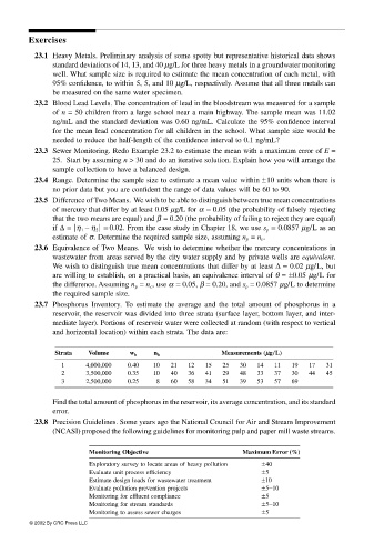
23.7 Phosphorus Inventory. To estimate the average and the total amount of phosphorus in a
reservoir, the reservoir was divided into three strata (surface layer, bottom layer, and inter-
mediate layer). Portions of reservoir water were collected at random (with respect to vertical
and horizontal location) within each strata. The data are:

Strata Volume w h n h Measurements (µµ µµg// //L)
1 4,000,000 0.40 10 21 12 15 25 30 14 11 19 17 31
2 3,500,000 0.35 10 40 36 41 29 48 33 37 30 44 45
3 2,500,000 0.25 8 60 58 34 51 39 53 57 69

Find the total amount of phosphorus in the reservoir, its average concentration, and its standard
error.
23.8 Precision Guidelines. Some years ago the National Council for Air and Stream Improvement
(NCASI) proposed the following guidelines for monitoring pulp and paper mill waste streams.

Monitoring Objective Maximum Error (%)
Exploratory survey to locate areas of heavy pollution ±40
Evaluate unit process efficiency ±5
Estimate design loads for wastewater treatment ±10
Evaluate pollution prevention projects ±5−10
Monitoring for effluent compliance ±5
Monitoring for stream standards ±5−10
Monitoring to assess sewer charges ±5
© 2002 By CRC Press LLC