Page 217 - Statistics for Environmental Engineers

L1592_frame_C24.fm Page 218 Tuesday, December 18, 2001 2:45 PM

TABLE 24.2
Analysis of Variance Table for Comparing Treatments A, B, and C
Source of Sum of Degrees of Mean F
Variation Squares Freedom Square Ratio
Between treatments 104 2 52 8.7
Within treatments 54 9 6
Total 158 11

Is the between-treatment variance larger than the within-treatment variance? This is judged by com-
paring the ratio of the between variance and the within variance. The ratios of sample variances are
distributed according to the F distribution. The tabulation of F values is arranged according to the degrees
of freedom in the variances used to compute the ratio. The numerator is the mean square of the “between-
treatments” variance, which has ν 1 degrees of freedom. The denominator is always the estimate of the
pure random error variance, in this case the “within-treatments” variance, which has ν 2 degrees of
freedom. An F value with these degrees of freedom is denoted by F ν 1 ,ν 2 ,α , where α is the upper percentage
point at which the test is being made. Usually α = 0.05 (5%) or α = 0.01 (1%). Geometrically, α is the
distribution that lies on the upper tail beyond the value F ν 1 ,ν 2 ,α .
area under the F ν 1 ,ν 2
The test will be made at the 5% level with degrees of freedom ν 1 = k − 1 = 3 − 1 = 2 and ν 2 = N −
k = 12 − 3 = 9. The relevant value is F 2,9,0.05 = 4.26. The ratio computed for our experiment, F = 52/6 =
8.67 is greater than F 2,9,α =0.05 = 4.26, so we conclude that σ b > σ w . This provides sufficient evidence to
2
2
conclude at the 95% confidence level that the means of the three treatments are not equal. We are entitled
only to conclude that η A ≠ η B ≠ η C . This analysis does not tell us whether one treatment is different
from the other two (i.e., η A ≠ η B but η B = η C ), or whether all three are different. To determine which
are different requires the kind of analysis described in Chapter 20.
When ANOVA is done by a commercial computer program, the results are presented in a special ANOVA
table that needs some explanation. For the example problem just presented, this table would be as given
in Table 24.2. The “sum of squares” in Table 24.2 is the sum of the squared deviations in the numerator
of each variance estimate. The “mean square” in Table 24.2 is the sum of squares divided by the degrees
2
of freedom of that sum of squares. The mean square values estimate the within-treatment variance (s w )
2
and the between-treatment variance (s b ). Note that the mean square for variation between treatments is
52, which is the between-treatment variance computed above. Also, note that the within treatment mean
square of 6 is the within-treatment variance computed above. The F ratio is the ratio of these two mean
squares and is the same as the F ratio of the two estimated variances computed above.

Case Study Solution

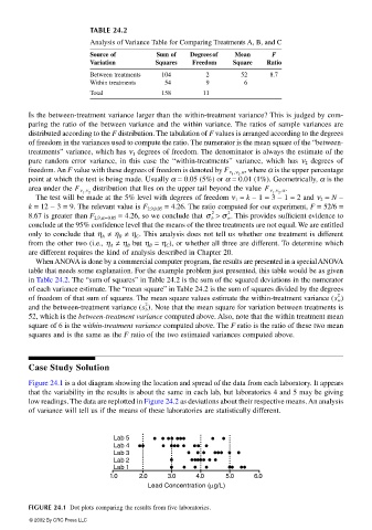
Figure 24.1 is a dot diagram showing the location and spread of the data from each laboratory. It appears
that the variability in the results is about the same in each lab, but laboratories 4 and 5 may be giving
low readings. The data are replotted in Figure 24.2 as deviations about their respective means. An analysis
of variance will tell us if the means of these laboratories are statistically different.

Lab 5
Lab 4
Lab 3
Lab 2
Lab 1
1.0 2.0 3.0 4.0 5.0 6.0
Lead Concentration (µg/L)

FIGURE 24.1 Dot plots comparing the results from five laboratories.
© 2002 By CRC Press LLC