Page 294 - Statistics for Environmental Engineers

L1592_frame_C33 Page 300 Tuesday, December 18, 2001 2:51 PM

2
The summation is over all squares of the settings of the independent variable x. σ is the experimental
error variance. (Warning: This equation does not give the variance for the slope of a two-parameter
linear model.)
2
Ideally, σ would be estimated from independent replicate experiments at some settings of the x
variable. There are no replicate measurements in our example, so another approach is used. The residual
2
sum of squares can be used to estimate σ if one is willing to assume that the model is correct. In this
case, the residuals are random errors and the average of these residuals squared is an estimate of the
(
error variance σ . Thus, σ may be estimated by dividing the residual sum of squares S R ) by its degrees
2
2
of freedom ν =( n – p), where n is the number of observations and p is the number of estimated
parameters.
In this example, S R = 0.0116, p = 1 parameter, n = 6, ν = 6 – 1 = 5 degrees of freedom, and the
estimate of the experimental error variance is:
s = ------------ = 0.0116 0.00232
2
---------------- =
S R
n – p 5
The estimated variance of b is:
2
s
Var b() = --------- = 0.00232 0.0000033
------------------- =
2 713
∑x i
and the standard error of b is:
SE b() = Var b() = 0.0000032 = 0.0018
The (1– α)100% confidence limits for the true value β are:

b ± t ν,α 2 SE b()
For α = 0.05, ν = 5, we find t 5,0.025 = 2.571 , and the 95% confidence limits are 0.1 ± 2.571(0.0018) =
0.1 ± 0.0046.
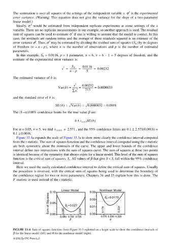
Figure 33.4a expands the scale of Figure 33.3a to show more clearly the confidence interval computed
from the t statistic. The sum of squares function and the confidence interval computed using the t statistic
are both symmetric about the minimum of the curve. The upper and lower bounds of the confidence
interval define two intersections with the sum of squares curve. The sum of squares at these two points
is identical because of the symmetry that always exists for a linear model. This level of the sum of squares
function is the critical sum of squares, S c . All values of β that give S < S c fall within the 95% confidence
interval.
Here we used the easily calculated confidence interval to define the critical sum of squares. Usually
the procedure is reversed, with the critical sum of squares being used to determine the boundary of
the confidence region for two or more parameters. Chapters 34 and 35 explain how this is done. The
F statistic is used instead of the t statistic.

Linear Model 0.03 Nonlinear Model
Sum of Squares 0.10 S = 0.027 0.02 0. 178 S = 0.0175 0.224
c
0.05
0.01
c
0.095
0.00
0.095 0.100 0.105 0. 105 0.00 0.175 0.200 0.225
β θ

FIGURE 33.4 Sum of squares functions from Figure 33.3 replotted on a larger scale to show the confidence intervals of
β for the linear model (left) and θ for the nonlinear model (right).
© 2002 By CRC Press LLC