Page 292 - Statistics for Environmental Engineers

L1592_frame_C33 Page 298 Tuesday, December 18, 2001 2:51 PM

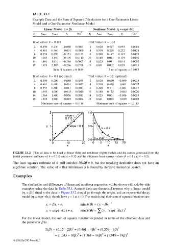
TABLE 33.1
Example Data and the Sum of Squares Calculations for a One-Parameter Linear
Model and a One-Parameter Nonlinear Model
Linear Model: ηη ηη == == ββ ββx Nonlinear Model: ηη ηη i == == exp(−θθ θθx i )
2 2
x i y obs,i y calc,i e i (e i ) x i y obs,i y calc,i e i (e i )
Trial value: b = 0.115 Trial value: k = 0.32
2 0.150 0.230 −0.080 0.0064 2 0.620 0.527 0.093 0.0086
4 0.461 0.460 0.001 0.0000 4 0.510 0.278 0.232 0.0538
6 0.559 0.690 −0.131 0.0172 6 0.260 0.147 0.113 0.0129
10 1.045 1.150 −0.105 0.0110 10 0.180 0.041 0.139 0.0194
14 1.364 1.610 −0.246 0.0605 14 0.025 0.011 0.014 0.0002
19 1.919 2.185 −0.266 0.0708 19 0.041 0.002 0.039 0.0015
Sum of squares = 0.1659 Sum of squares = 0.0963
Trial value: b = 0.1 (optimal) Trial value: k = 0.2 (optimal)
2 0.150 0.200 −0.050 0.0025 2 0.620 0.670 −0.050 0.0025
4 0.461 0.400 0.061 0.0037 4 0.510 0.449 0.061 0.0037
6 0.559 0.600 −0.041 0.0017 6 0.260 0.301 −0.041 0.0017
10 1.045 1.000 0.045 0.0020 10 0.180 0.135 0.045 0.0020
14 1.364 1.400 −0.036 0.0013 14 0.025 0.061 −0.036 0.0013
19 1.919 1.900 0.019 0.0004 19 0.041 0.022 0.019 0.0003
Minimum sum of squares = 0.0116 Minimum sum of squares = 0.0115

2 1.0
slope =
0.115

y 1 slope = 0.1 0.5
k = 0.2

k = 0.32
0 0.0
0 10 20 0 5 10 15 20
x x
FIGURE 33.2 Plots of data to be fitted to linear (left) and nonlinear (right) models and the curves generated from the
initial parameter estimates of b = 0.115 and k = 0.32 and the minimum least squares values (b = 0.1 and k = 0.2).

The least squares estimate of θ still satisfies ∂S/∂θ = 0, but the resulting derivative does not have an
algebraic solution. The value of θ that minimizes S is found by iterative numerical search.
Examples

The similarities and differences of linear and nonlinear regression will be shown with side-by-side
examples using the data in Table 33.1. Assume there are theoretical reasons why a linear model
(η i = βx i ) fitted to the data in Figure 33.2 should go through the origin, and an exponential decay
model (η i = exp( −θx i )) should have y = 1 at t = 0. The models and their sum of squares functions are:

y i = βx i + e i min S β() = ( y i βx i ) 2
–
– (
y i = exp – ( θx i ) + e i min S θ() = ∑ ( y i – exp θx i )) 2
For the linear model, the sum of squares function expanded in terms of the observed data and
the parameter β is:
S β() = ( 0.15 2β) + ( 0.461 4β) + ( 0.559 6β) 2
2
2
–
–
–
+ ( 1.045 10β– ) + ( 1.361 14β) + ( 1.919 19β) 2
2
2
–
–
© 2002 By CRC Press LLC