Page 287 - Statistics for Environmental Engineers

L1592_frame_C32 Page 292 Tuesday, December 18, 2001 2:50 PM

Implications for Sampling Frequency
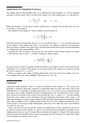
The sample mean of autocorrelated data (y) is unaffected by autocorrelation. It is still an unbiased
estimator of the true mean. This is not true of the variance of y or the sample mean y, as calculated by:

(
s y = ∑ y t – y) 2 and s y = s y /n
2
2
2
------------------------
n 1
–
2
With autocorrelation, s y is the purely random variation plus a component due to drift about the mean
(or perhaps a cyclic pattern).
y
The estimate of the variance of that accounts for autocorrelation is:
2 2 n−1
2 ∑
s y = ---- + 2s y ( n 1) r k
2
s y
–
-------
n n
k=1
If the observations are independent, then all r k are zero and this becomes s y = s y /n, the usual expression
2
2
for the variance of the sample mean. If the r k are positive (>0), which is common for environmental
data, the variance is inflated. This means that n correlated observations will not give as much information
as n independent observations (Gilbert, 1987).
Assuming the data vary about a fixed mean level, the number of observations required to estimate
y with maximum error E and (1 − α )100% confidence is approximately:
2

∑
n =   z α/2 σ  1 + 2 n−1 r k 
------------ 
E 

k=1 
The lag at which r k becomes negligible identifies the time between samples at which observations become
independent. If we sample at that interval, or at a greater interval, the sample size needed to estimate
2
the mean is reduced to n = (z α/2 σ/E ) .
If there is a regular cycle, sample at half the period of the cycle. For a 24-h cycle, sample every 12 h.
If you sample more often, select multiples of the period (e.g., 6 h, 3 h).
Comments
Undetected serial correlation, which is a distinct possibility in small samples (n < 50), can be very
upsetting to statistical conclusions, especially to conclusions based on t-tests and F-tests. This is why
randomization is so important in designed experiments. The t-test is based on an assumption that the
observations are normally distributed, random, and independent. Lack of independence (serial correla-
tion) will bias the estimate of the variance and invalidate the t-test. A sample of n = 20 autocorrelated
observations may contain no more information than ten independent observations. Thus, using n = 20
makes the test appear to be more sensitive than it is. With moderate autocorrelation and moderate sample
sizes, what you think is a 95% confidence interval may be in fact a 75% confidence interval. Box et al.
(1978) present a convincing example. Montgomery and Loftis (1987) show how much autocorrelation
can distort the error rate.
Linear regression also assumes that the residuals are independent. If serial correlation exists, but we
are unaware and proceed as though it is absent, all statements about probabilities (hypothesis tests,
confidence intervals, etc.) may be wrong. This is illustrated in Chapter 41. Chapter 54 on intervention
analysis discusses this problem in the context of assessing the shift in the level of a time series related
to an intentional intervention in the system.

© 2002 By CRC Press LLC