Page 285 - Statistics for Environmental Engineers

L1592_frame_C32 Page 290 Tuesday, December 18, 2001 2:50 PM

TABLE 32.1
120 BOD Observations Made at 2-h Intervals
Sampling Interval
Day 1 2 3 4 5 6 7 8 9 10 11 12
1 200 122 153 176 129 168 165 119 113 110 113 98
2 180 122 156 185 163 177 194 149 119 135 113 129
3 160 105 127 162 132 184 169 160 115 105 102 114
4 112 148 217 193 208 196 114 138 118 126 112 117
5 180 160 151 88 118 129 124 115 132 190 198 112
6 132 99 117 164 141 186 137 134 120 144 114 101
7 140 120 182 198 171 170 155 165 131 126 104 86
8 114 83 107 162 140 159 143 129 117 114 123 102
9 144 143 140 179 174 164 188 107 140 132 107 119
10 156 116 179 189 204 171 141 123 117 98 98 108
Note: Time runs left to right.

250
BOD (mg/L) 200

150
100
50
0 24 48 72 96 120 144 168 192 216 240
Hours

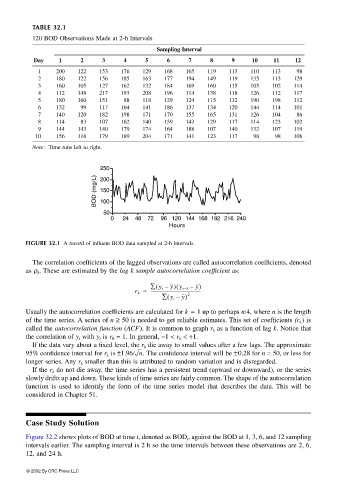
FIGURE 32.1 A record of influent BOD data sampled at 2-h intervals.

The correlation coefficients of the lagged observations are called autocorrelation coefficients, denoted
as ρ k . These are estimated by the lag k sample autocorrelation coefficient as:
(
(
r k = ∑ y t – y) y t−k – y)
--------------------------------------------
∑ y t –( y) 2
Usually the autocorrelation coefficients are calculated for k = 1 up to perhaps n/4, where n is the length
of the time series. A series of n ≥ 50 is needed to get reliable estimates. This set of coefficients (r k ) is
called the autocorrelation function (ACF). It is common to graph r k as a function of lag k. Notice that
the correlation of y t with y t is r 0 = 1. In general, −1 < r k < +1.
If the data vary about a fixed level, the r k die away to small values after a few lags. The approximate
95% confidence interval for r k is ±1.96/ n . The confidence interval will be ±0.28 for n = 50, or less for
longer series. Any r k smaller than this is attributed to random variation and is disregarded.
If the r k do not die away, the time series has a persistent trend (upward or downward), or the series
slowly drifts up and down. These kinds of time series are fairly common. The shape of the autocorrelation
function is used to identify the form of the time series model that describes the data. This will be
considered in Chapter 51.

Case Study Solution
Figure 32.2 shows plots of BOD at time t, denoted as BOD t , against the BOD at 1, 3, 6, and 12 sampling
intervals earlier. The sampling interval is 2 h so the time intervals between these observations are 2, 6,
12, and 24 h.

© 2002 By CRC Press LLC