Page 288 - Statistics for Environmental Engineers

L1592_frame_C32 Page 293 Tuesday, December 18, 2001 2:50 PM

References
Box, G. E. P., W. G. Hunter, and J. S. Hunter (1978). Statistics for Experimenters: An Introduction to Design,
Data Analysis, and Model Building, New York, Wiley Interscience.
Box, G. E. P., G. M. Jenkins, and G. C. Reinsel (1994). Time Series Analysis, Forecasting and Control, 3rd
ed., Englewood Cliffs, NJ, Prentice-Hall.
Cryer, J. D. (1986). Time Series Analysis, Boston, MA, Duxbury Press.
Gilbert, R. O. (1987). Statistical Methods for Environmental Pollution Monitoring, New York, Van Nostrand
Reinhold.
Montgomery, R. H. and J. C. Loftis, Jr. (1987). “Applicability of the t-Test for Detecting Trends in Water
Quality Variables,” Water Res. Bull., 23, 653–662.

Exercises

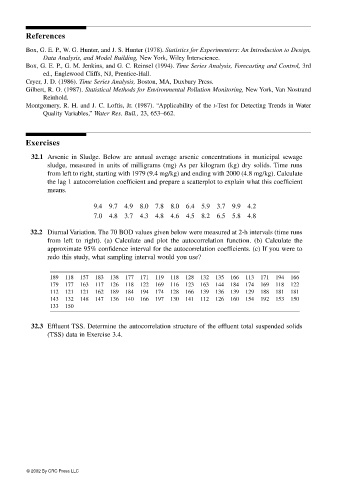
32.1 Arsenic in Sludge. Below are annual average arsenic concentrations in municipal sewage
sludge, measured in units of milligrams (mg) As per kilogram (kg) dry solids. Time runs
from left to right, starting with 1979 (9.4 mg/kg) and ending with 2000 (4.8 mg/kg). Calculate
the lag 1 autocorrelation coefficient and prepare a scatterplot to explain what this coefficient
means.
9.4 9.7 4.9 8.0 7.8 8.0 6.4 5.9 3.7 9.9 4.2
7.0 4.8 3.7 4.3 4.8 4.6 4.5 8.2 6.5 5.8 4.8

32.2 Diurnal Variation. The 70 BOD values given below were measured at 2-h intervals (time runs
from left to right). (a) Calculate and plot the autocorrelation function. (b) Calculate the
approximate 95% confidence interval for the autocorrelation coefficients. (c) If you were to
redo this study, what sampling interval would you use?

189 118 157 183 138 177 171 119 118 128 132 135 166 113 171 194 166
179 177 163 117 126 118 122 169 116 123 163 144 184 174 169 118 122
112 121 121 162 189 184 194 174 128 166 139 136 139 129 188 181 181
143 132 148 147 136 140 166 197 130 141 112 126 160 154 192 153 150
133 150

32.3 Effluent TSS. Determine the autocorrelation structure of the effluent total suspended solids
(TSS) data in Exercise 3.4.

© 2002 By CRC Press LLC