Page 293 - Statistics for Environmental Engineers

L1592_frame_C33 Page 299 Tuesday, December 18, 2001 2:51 PM

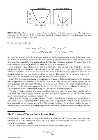
Linear Model Nonlinear Model
0.3
Sum of Squares 0.2 b =0.1 k = 0.2

0.1

0.0
0.09 0.10 0.11 0.1 0.2 0.3
β θ

FIGURE 33.3 The values of the sum of squares plotted as a function of the trial parameter values. The least squares
estimates are b = 0.1 and k = 0.2. The sum of squares function is symmetric (parabolic) for the linear model (left) and
asymmetric for the nonlinear model (right).

For the nonlinear model it is:

) +
6θ 2
) +
S θ() = ( 0.62 e – 2θ 2 ( 0.51 e – 4θ 2 ( 0.26 e )
–
–
–
)
+ ( 0.18 e – 10θ 2 ( 0.025 e – 14θ 2 ( 0.041 e – 19θ 2
–
–
) +
–
) +
An algebraic solution exists for the linear model, but to show the essential similarity between linear
and nonlinear parameter estimation, the least squares parameter estimates of both models will be
determined by a straightforward numerical search of the sum of squares functions. We simply plot S β()
over a range of values of β, and do the same for S θ() over a range of θ.
Two iterations of this calculation are shown in Table 33.1. The top part of the table shows the trial
calculations for initial parameter estimates of b = 0.115 and k = 0.32. One clue that these are poor
estimates is that the residuals are not random; too many of the linear model regression residuals are
negative and all the nonlinear model residuals are positive. The bottom part of the table is for b = 0.1
and k = 0.2, the parameter values that give the minimum sum of squares.
Figure 33.3 shows the smooth sum of squares curves obtained by following this approach. The minimum
sum of squares — the minimum point on the curve — is called the residual sum of squares and the
corresponding parameter values are called the least squares estimates. The least squares estimate of
y ˆ
y ˆ
β is b = 0.1. The least squares estimate of θ is k = 0.2. The fitted models are = 0.1x and = exp( −0.2x).
y ˆ is the predicted value of the model using the least squares parameter estimate.
The sum of squares function of a linear model is always symmetric. For a univariate model it will be
a parabola. The curve in Figure 33.3a is a parabola. The sum of squares function for nonlinear models
is not symmetric, as can be seen in Figure 33.3b.
When a model has two parameters, the sum of squares function can be drawn as a surface in three
dimensions, or as a contour map in two dimensions. For a two-parameter linear model, the surface will
be a parabaloid and the contour map of S will be concentric ellipses. For nonlinear models, the sum of
squares surface is not defined by any regular geometric function and it may have very interesting contours.

The Precision of Estimates of a Linear Model

Calculating the “best” values of the parameters is only part of the job. The precision of the parameter
estimates needs to be understood. Figure 33.3 is the basis for showing the confidence interval of the
example one-parameter models.
For the one-parameter linear model through the origin, the variance of b is:

σ 2
Var b() = ---------
2
∑x i
© 2002 By CRC Press LLC