Page 297 - Statistics for Environmental Engineers

L1592_frame_C34 Page 303 Tuesday, December 18, 2001 2:52 PM
34

Precision of Parameter Estimates in Linear Models

KEY WORDS confidence interval, critical sum of squares, joint confidence region, least squares, linear
regression, mean residual sum of squares, nonlinear regression, parameter correlation, parameter estima-
tion, precision, prediction interval, residual sum of squares, straight line.

Calculating the best values of the parameters is only half the job of fitting and evaluating a model. The
precision of these estimates must be known and understood. The precision of estimated parameters in
a linear or nonlinear model is indicated by the size of their joint confidence region. Joint indicates that
all the parameters in the model are considered simultaneously.

The Concept of a Joint Confidence Region
When we fit a model, such as η = β 0 + β 1 x or η = θ 1 [1 − exp(−θ 2 x)], the regression procedure delivers
a set of parameter values. If a different sample of data were collected using the same settings of x,
different y values would result and different parameter values would be estimated. If this were repeated
with many data sets, many pairs of parameter estimates would be produced. If these pairs of parameter
estimates were plotted as x and y on Cartesian coordinates, they would cluster about some central point
that would be very near the true parameter values. Most of the pairs would be near this central value,
but some could fall a considerable distance away. This happens because of random variation in the y
measurements.
The data (if they are useful for model building) will restrict the plausible parameter values to lie within
a certain region. The intercept and slope of a straight line, for example, must be within certain limits or
the line will not pass through the data, let alone fit it reasonably well. Furthermore, if the slope is
decreased somewhat in an effort to better fit the data, inevitably the intercept will increase slightly to
preserve a good fit of the line. Thus, low values of slope paired with high values of intercept are plausible,
but high slopes paired with high intercepts are not. This relationship between the parameter values is
called parameter correlation. It may be strong or weak, depending primarily on the settings of the x
variables at which experimental trials are run.
Figure 34.1 shows some joint confidence regions that might be observed for a two-parameter model.
Panels (a) and (b) show typical elliptical confidence regions of linear models; (c) and (d) are for nonlinear
models that may have confidence regions of irregular shape. A small joint confidence region indicates
precise parameter estimates. The orientation and shape of the confidence region are also important. It
may show that one parameter is estimated precisely while another is only known roughly, as in (b) where
β 2 is estimated more precisely than β 1 . In general, the size of the confidence region decreases as the
number of observations increases, but it also depends on the actual choice of levels at which measure-
ments are made. This is especially important for nonlinear models. The elongated region in (d) could
result from placing the experimental runs in locations that are not informative.
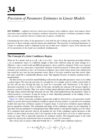
The critical sum of squares value that bounds the (1 − α)100% joint confidence region is:




p
p
S c = S R + S R ------------ F p,n− p,α = S R 1 + ------------ F p,n− p,α  



p
n –
p
n –
© 2002 By CRC Press LLC