Page 302 - Statistics for Environmental Engineers

L1592_frame_C34 Page 308 Tuesday, December 18, 2001 2:52 PM

2.0
1.5 Interval estimates
of the confidence
1.0 region
b 0.5
2
95% joint
0 confidence region
-0.5
-1.0
130 140 150
b
1
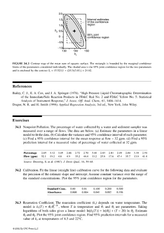
FIGURE 34.3 Contour map of the mean sum of squares surface. The rectangle is bounded by the marginal confidence
limits of the parameters considered individually. The shaded area is the 95% joint confidence region for the two parameters
and is enclosed by the contour S c = 15.523[1 + (2/13)(3.81)] = 24.62.

References

Bailey, C. J., E. A. Cox, and J. A. Springer (1978). “High Pressure Liquid Chromatographic Determination
of the Immediate/Side Reaction Products in FD&C Red No. 2 and FD&C Yellow No. 5: Statistical
Analysis of Instrument Response,” J. Assoc. Off. Anal. Chem., 61, 1404–1414.
Draper, N. R. and H. Smith (1998). Applied Regression Analysis, 3rd ed., New York, John Wiley.

Exercises
34.1 Nonpoint Pollution. The percentage of water collected by a water and sediment sampler was
measured over a range of flows. The data are below. (a) Estimate the parameters in a linear
model to fit the data. (b) Calculate the variance and 95% confidence interval of each parameter.
(c) Find a 95% confidence interval for the mean response at flow = 32 gpm. (d) Find a 95%
prediction interval for a measured value of percentage of water collected at 32 gpm.

Percentage 2.65 3.12 3.05 2.86 2.72 2.70 3.04 2.83 2.84 2.49 2.60 3.19 2.54
Flow (gpm) 52.1 19.2 4.8 4.9 35.2 44.4 13.2 25.8 17.6 47.4 35.7 13.9 41.4
Source: Dressing, S. et al. (1987). J. Envir. Qual., 16, 59–64.

34.2 Calibration. Fit the linear (straight line) calibration curve for the following data and evaluate
the precision of the estimate slope and intercept. Assume constant variance over the range of
the standard concentrations. Plot the 95% joint confidence region for the parameters.

Standard Conc. 0.00 0.01 0.100 0.200 0.500
Absorbance 0.000 0.004 0.041 0.082 0.196

34.3 Reaeration Coefficient. The reaeration coefficient (k 2 ) depends on water temperature. The
T −20
model is k 2 (T ) = θ 1 θ 2 , where T is temperature and θ 1 and θ 2 are parameters. Taking
logarithms of both sides gives a linear model: ln[k 2 (T )] = ln[θ 1 ] + (T − 20) ln θ 2 . Estimate
θ 1 and θ 2 . Plot the 95% joint confidence region. Find 95% prediction intervals for a measured
value of k 2 at temperatures of 8.5 and 22°C.

© 2002 By CRC Press LLC