Page 306 - Statistics for Environmental Engineers

L1592_frame_C35 Page 313 Tuesday, December 18, 2001 2:52 PM

of substrate concentration would not help very much. Often the best way to shrink the size of the
confidence region is to be more intelligent about selecting the settings of the independent variable at
which observations will be made. Examples are given in the next two sections to illustrate this.

Do More Observations Improve Precision?
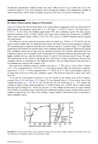
Figure 35.2 shows the Monod model fitted to the original data set augmented with two observations at
high substrate concentrations, specifically at (x = 225 mg/L, y = 0.122 h ) and (x = 375 mg/L and y =
−1
−1
0.125 h ). It also shows the resulting approximate 95% joint confidence region. The least squares
ˆ
parameter estimates are 1 = 0.146 h and 2 = 49.1 mg/L, with a residual sum of squares S R = 0.000817.θ −1 θ
ˆ
These values compare closely with 1 = 0.153, 2 = 55.4, and S R = 0.00079 obtained with the originalθ θ
ˆ
ˆ
five observations.
The differences in the estimated parameter values are small (e.g., 0.146 vs. 0.153 for ) and oneθ ˆ 1
might wonder whether the two additional observations did lead to more precise parameter estimates.
The substantial gain is apparent when the joint confidence region is examined. Figure 35.2 (right-hand
panel) shows that both the size and the shape of the confidence region are improved. Whereas the original
joint confidence region was so large that the parameter estimates were virtually unbounded, the joint
confidence region is now reasonably small. In particular, θ 1 is estimated with good precision and we are
highly confident the true value lies between about 0.1 and 0.2. θ 2 is between about 30 and 150 mg/L.
The improvement is due mainly to having the new observations at large concentrations because they
contribute directly to estimating θ 1 . The additional benefit is that any improvement in the precision of
θ 1 simultaneously improves the estimate of θ 2 .
One reason the confidence region is smaller is because n = 7. This gives a value of the F statistic
of F = 5.79, compared with F = 9.55 for n = 5. The sum of squares value that bounds the confidence
region for n = 7 is S c = 3.316S R compared with S c = 7.367S R for n = 5. This would explain a reduction
of about half in the size of the joint confidence region. The observed reduction is many times more
than this.
To see that the improvement in precision is not due entirely to the smaller value of the F statistic,
compare Figure 35.1 with Figure 35.3. Figure 35.3 was obtained from n = 5 observations (four of the
original data points at x = 28, 55, 83, and 138 plus the one new observation at x = 375). Indeed, the
confidence region is larger, being bounded by S c = 0.0057 instead of S c = 0.0027, but it is much smaller
than the region in Figure 35.1, which was also for n = 5 but without an observation at a high substrate
level. Clearly, it is possible to get a small and well-conditioned confidence region without doing a massive
number of experiments. Also clear is the corollary: a large number of observations does not guarantee a
small confidence region.

0.15 200
0. 005 0.0027 005 150
Growth Rate (1/h) 0.05 θ = 0.146 Approximate 100 θ 2
0.10
S = 0.000817
0.
R
^
1
^
θ = 49.1
2
50
95% joint
confidence
region
0 0
0 100 200 300 400 0 0.10 0.2 0.3 0.4
Substrate Concentration (mg/L) θ 1
FIGURE 35.2 Monod model fitted to the original five points plus two more at higher substrate concentrations (left) and
the resulting joint confidence region of the parameters (right).
© 2002 By CRC Press LLC