Page 307 - Statistics for Environmental Engineers

L1592_frame_C35 Page 314 Tuesday, December 18, 2001 2:52 PM

0. 15 200
0.05 0. 05 150
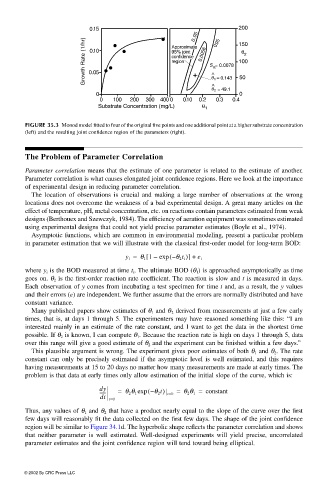
Growth Rate (1/hr) 0.05 95% joint 0.0058 S = 0.0078 100
Approximate
θ
0.10
2
confidence
region
R
^
θ
θ ^ 1 = 0.143 50
2 = 49.1
0 0
0 100 200 300 400 0 0.10 0.2 0.3 0.4
Substrate Concentration (mg/L) θ 1
FIGURE 35.3 Monod model fitted to four of the original five points and one additional point at a higher substrate concentration
(left) and the resulting joint confidence region of the parameters (right).

The Problem of Parameter Correlation

Parameter correlation means that the estimate of one parameter is related to the estimate of another.
Parameter correlation is what causes elongated joint confidence regions. Here we look at the importance
of experimental design in reducing parameter correlation.
The location of observations is crucial and making a large number of observations at the wrong
locations does not overcome the weakness of a bad experimental design. A great many articles on the
effect of temperature, pH, metal concentration, etc. on reactions contain parameters estimated from weak
designs (Berthouex and Szewczyk, 1984). The efficiency of aeration equipment was sometimes estimated
using experimental designs that could not yield precise parameter estimates (Boyle et al., 1974).
Asymptotic functions, which are common in environmental modeling, present a particular problem
in parameter estimation that we will illustrate with the classical first-order model for long-term BOD:
y i = θ 1 1 – exp – ( θ 2 t i )] + e i
[
where y i is the BOD measured at time t i . The ultimate BOD (θ 1 ) is approached asymptotically as time
goes on. θ 2 is the first-order reaction rate coefficient. The reaction is slow and t is measured in days.
Each observation of y comes from incubating a test specimen for time t and, as a result, the y values
and their errors (e) are independent. We further assume that the errors are normally distributed and have
constant variance.
Many published papers show estimates of θ 1 and θ 2 derived from measurements at just a few early
times, that is, at days 1 through 5. The experimenters may have reasoned something like this: “I am
interested mainly in an estimate of the rate constant, and I want to get the data in the shortest time
possible. If θ 2 is known, I can compute θ 1 . Because the reaction rate is high on days 1 through 5, data
over this range will give a good estimate of θ 2 and the experiment can be finished within a few days.”
This plausible argument is wrong. The experiment gives poor estimates of both θ 1 and θ 2 . The rate
constant can only be precisely estimated if the asymptotic level is well estimated, and this requires
having measurements at 15 to 20 days no matter how many measurements are made at early times. The
problem is that data at early times only allow estimation of the initial slope of the curve, which is:

dy = – ( θ 2 t) = θ 2 θ 1 =
------ θ 2 θ 1 exp t=0 constant
dt t=0
Thus, any values of θ 1 and θ 2 that have a product nearly equal to the slope of the curve over the first
few days will reasonably fit the data collected on the first few days. The shape of the joint confidence
region will be similar to Figure 34.1d. The hyperbolic shape reflects the parameter correlation and shows
that neither parameter is well estimated. Well-designed experiments will yield precise, uncorrelated
parameter estimates and the joint confidence region will tend toward being elliptical.

© 2002 By CRC Press LLC