Page 312 - Statistics for Environmental Engineers

L1592_frame_C36.fm Page 320 Tuesday, December 18, 2001 3:20 PM
TABLE 36.1
Calibration Data for HPLC Measurement of Dye
Dye Conc. 0.18 0.35 0.055 0.022 0.29 0.15 0.044 0.028
HPLC Peak Area 26.666 50.651 9.628 4.634 40.206 21.369 5.948 4.245
Dye Conc. 0.044 0.073 0.13 0.088 0.26 0.16 0.10
HPLC Peak Area 4.786 11.321 18.456 12.865 35.186 24.245 14.175
Note: In run order reading from left to right.
Source: Bailey, C. J., E. A. Cox, and J. A. Springer (1978). J. Assoc. Off. Anal. Chem., 61, 1404–1414; Hunter,
J. S. (1981). J. Assoc. Off. Anal. Chem., 64(3), 574–583.

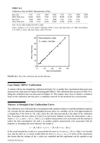
50 Fitted calibration model
^
y = 0.556 + 139.759x
40
HPLC Peak Area 30

20

10

0
0 0.1 0.2 0.3 0.4
Dye Concentration

FIGURE 36.1 Plot of the calibration data and the fitted line.

Case Study: HPLC Calibration
A chemist will use the straight-line calibration in Figure 36.1 to predict dye concentration from peak areas
measured on a high-pressure liquid chromatograph (HPLC). The calibration data are given in Table 36.1;
fitting the calibration line was discussed in Chapter 34. This chapter shows how to obtain a confidence
band for the calibration line that gives a confidence interval for the predicted dye concentration.

Theory: A Straight-Line Calibration Curve

The calibration curve will relate the concentration of the standard solution (x) and the instrument response
(η). Assume that the functional relationship between these two variables can be well approximated by
a straight line of the form η = β 0 + β 1 ξ, where β 0 is the intercept and β 1 is the slope of the calibration
line. In practice, the true values of η and ξ are not known. Instead, we have the observations x and y,
where x = ξ + e x and y = η + e y . Here e x is a random measurement error associated with the attempt to
realize the true concentration (ξ ) and e y is another random measurement error associated with the
response η. Assuming this error structure, the model is:
(
y = β 0 + β 1 x – e x ) + e y = β 0 + β 1 x + ( e y β 1 e x )
–
In the usual straight-line model, it is assumed that the error in x is zero (e x = 0) or, if that is not literally
true, that the error in x is much smaller than the error in y (i.e., e x << e y ). In terms of the experiment,
this means that the settings of the x values are controlled and the experiment can be repeated at any
© 2002 By CRC Press LLC