Page 315 - Statistics for Environmental Engineers

L1592_frame_C36.fm Page 323 Tuesday, December 18, 2001 3:20 PM

The specific steps to construct the Working-Hotelling confidence band and confidence interval are as
follows. The measured peak area of 22.0 yields an estimated concentration of 0.153. The confidence
limits for the y value that will contain the true value of the peak area (ordinate) 90% of the time are
calculated using z p=0.9 = 1.28. To have a confidence level of 100(1 − α )% = 95%, specify α/2 = 0.025,
2
which gives χ 13,0.025 = 5.01 . The corresponding interval for the peak area is:

13 1.194)
(
y ± 1.28 ------------------------ = y ± 2.253
5.01
For the observed peak area (y = 22.0), the relevant interval estimate of the ordinate variable is 22 ± 2.253.
Or, we can state with 95% confidence that the bounds:
19.75 ≤ η ≤ 24.25

contain the true value of peak area 90% of the time.
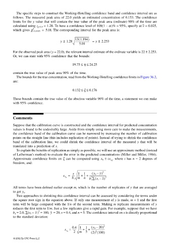
The bounds for the true concentration, read from the Working-Hotelling confidence limits in Figure 36.2,
are:

ξ
0.132 ≤≤ 0.176
These bounds contain the true value of the abscissa variable 90% of the time, a statement we can make
with 95% confidence.

Comments
Suppose that the calibration curve is constructed and the confidence interval for predicted concentration
values is found to be undesirably large. Aside from simply using more care to make the measurements,
the confidence band of the calibration curve can be narrowed by increasing the number of calibration
points on the straight line (this includes replication of points). Instead of trying to shrink the confidence
band of the calibration line, we could shrink the confidence interval of the measured y that will be
translated into a prediction of x.
To explain the benefits of replication as simply as possible, we will use an approximate method (instead
of Leiberman’s method) to evaluate the error in the predicted concentrations (Miller and Miller, 1984).
, where t has n − 2 degrees of
Approximate confidence limits on ξ can be computed using x 0 ± ts x 0
freedom, and:

y)
(
2
y 0 –
1
s
= ----- ---- + 1 --- + -----------------------------
(
b 1 m n b 1 ∑ x i – x)
s x 0 2 2
All terms have been defined earlier except m, which is the number of replicates of y that are averaged
to get y o .
Two approaches to shrinking this confidence interval can be assessed by considering the terms under
the square root sign in the equation above. If only one measurement of y is made, m = 1 and the first
term will be large compared with the 1/n of the second term. Making m replicate measurements of y
reduces the first term to 1/m. Just a few replicates give a rapid gain. For example, suppose that we have
b 1 = 2.0, ∑(x i − ) = 100, = 20, s = 0.4, and n = 5. The confidence interval on x is directly proportionalx 2 y
to the standard deviation:
20)
y 0 –
------- ---- +
= 0.4 1 1 --- + ( ------------------------ 2
(
2 m 5 2 () 100)
s x 0 2
© 2002 By CRC Press LLC