Page 313 - Statistics for Environmental Engineers

L1592_frame_C36.fm Page 321 Tuesday, December 18, 2001 3:20 PM

desired x value. In most calibration problems, it is accepted that the random variability of the measurement
system can be attributed solely to the y values. Thus, the model becomes the familiar:

y = β 0 + β 1 x + e y
Usually the e y are assumed to be independent and normally distributed with mean zero and constant
2
variance σ .
It is now clear that fitting the best straight-line calibration curve is a problem of linear regression. The
slope and intercept of the straight line are estimated and their precision is evaluated using the procedures
described in Chapter 34. An excellent summary of single component calibration is given by Danzer and
Currie (1998).

Using the Calibration Curve

In practice, the objective is to estimate concentrations (x values) from measured peak areas (y values).
The calibration curve is a means to this end. This is the inverse prediction problem; that is, the inverse
of the common use of a fitted model to predict y from a known value of x.
An interesting problem arises in using the calibration curve in this inverse fashion. Of course it is a
simple matter to use the fitted equation (y = b 0 + b 1 x) to compute x for any given value of y. Specifically,
the estimate of x for any future observation y is x ˆ = ( yb 0 )/b 1 . Because the calibration curve is to be
–
used over and over again, what is required for a future value of y, in addition to the predicted value , x ˆ
is an interval estimate that has the property that at least 100P% of the intervals will contain the true
concentration value ξ with 100(1 − α)% confidence. For example, for P = 0.9 and α = 0.05, we can
assert with 95% confidence that 90% of the computed interval estimates of concentration will contain
the true value. This problem was resolved by Leiberman et al. (1967). Hunter (1981) gives details.
The error in clearly will depend in some way on the error in measuring y and on how closely b 0 and
x ˆ
b 1 estimate the true slope and intercept of the calibration line. The uncertainties associated with estimating
β 0 and β 1 imply that the regression line is not unique. Another set of standards and measurements would
yield a different line. We should consider, instead of a regression line, that there is a regression band (Sharaf
et al., 1986), which can be represented by a confidence band for the calibration line. The confidence band
for the entire calibration line (i.e., valid for any value of x) can be used to translate the confidence interval
for the true response η, based on a future observation of y, into a confidence interval for the abcissa value.
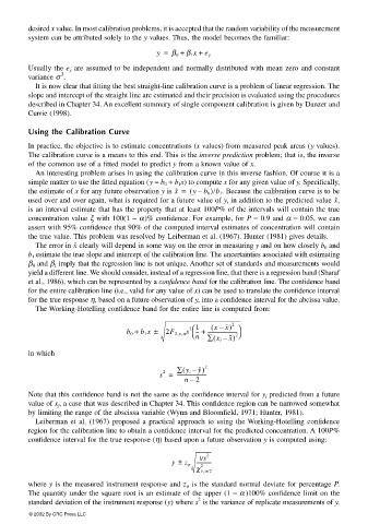
The Working-Hotelling confidence band for the entire line is computed from:
(
x)
2

2 1
x –
b 0 + b 1 x ± 2F 2,ν,α s --- + ------------------------ 
n  ∑ x i – x) 2 
(
in which
∑ y i y ˆ) 2
(
–
s = ------------------------
2
n 2
–
Note that this confidence band is not the same as the confidence interval for y f predicted from a future
value of x f , a case that was described in Chapter 34. This confidence region can be narrowed somewhat
by limiting the range of the abscissa variable (Wynn and Bloomfield, 1971; Hunter, 1981).
Leiberman et al. (1967) proposed a practical approach to using the Working-Hotelling confidence
region for the calibration line to obtain a confidence interval for the predicted concentration. A 100P%
confidence interval for the true response (η) based upon a future observation y is computed using:
2
νs
y ± z p ------------
2
χ ν,α/2
where y is the measured instrument response and z p is the standard normal deviate for percentage P.
The quantity under the square root is an estimate of the upper (1 − α )100% confidence limit on the
2
standard deviation of the instrument response (y) where s is the variance of replicate measurements of y.
© 2002 By CRC Press LLC