Page 317 - Statistics for Environmental Engineers

L1592_frame_C36.fm Page 325 Tuesday, December 18, 2001 3:20 PM

Exercises
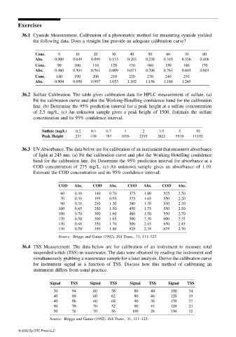
36.1 Cyanide Measurement. Calibration of a photometric method for measuring cyanide yielded
the following data. Does a straight line provide an adequate calibration curve?

Conc. 0 10 20 30 40 50 60 70 80
Abs. 0.000 0.049 0.099 0.153 0.203 0.258 0.310 0.356 0.406
Conc. 90 100 110 120 130 140 150 160 170
Abs. 0.460 0.504 0.561 0.609 0.671 0.708 0.761 0.803 0.863
Conc. 180 190 200 210 220 230 240 250
Abs. 0.904 0.956 0.997 1.053 1.102 1.158 1.186 1.245

36.2 Sulfate Calibration. The table gives calibration data for HPLC measurement of sulfate. (a)
Fit the calibration curve and plot the Working-Hotelling confidence band for the calibration
line. (b) Determine the 95% prediction interval for a peak height at a sulfate concentration
of 2.5 mg/L. (c) An unknown sample gives a peak height of 1500. Estimate the sulfate
concentration and its 95% confidence interval.

Sulfate (mg/L) 0.2 0.4 0.7 1 2 3.5 5 10
Peak Height 237 438 787 1076 2193 3821 5519 11192

36.3 UV Absorbance. The data below are for calibration of an instrument that measures absorbance
of light at 245 nm. (a) Fit the calibration curve and plot the Working-Hotelling confidence
band for the calibration line. (b) Determine the 95% prediction interval for absorbance at a
COD concentration of 275 mg/L. (c) An unknown sample gives an absorbance of 1.10.
Estimate the COD concentration and its 95% confidence interval.

COD Abs. COD Abs. COD Abs. COD Abs.
60 0.30 140 0.70 375 1.80 525 2.50
70 0.30 195 0.95 375 1.65 550 2.20
90 0.35 250 1.30 380 1.70 550 2.30
100 0.45 250 1.50 450 1.75 550 2.50
100 0.70 300 1.60 480 1.50 550 2.70
120 0.50 300 1.65 500 2.30 600 2.35
130 0.48 350 1.70 500 2.45 650 2.45
130 0.70 350 1.80 525 2.35 675 2.70
Source: Briggs and Gatter (1992). ISA Trans., 31, 111–123.

36.4 TSS Measurement. The data below are for calibration of an instrument to measure total
suspended solids (TSS) in wastewater. The data were obtained by reading the instrument and
simultaneously grabbing a wastewater sample for a later analysis. Derive the calibration curve
for instrument signal as a function of TSS. Discuss how this method of calibrating an
instrument differs from usual practice.

Signal TSS Signal TSS Signal TSS Signal TSS
30 94 60 58 80 40 100 34
40 80 60 62 80 46 120 19
40 86 60 68 90 38 120 22
50 70 70 52 90 41 120 23
50 76 70 56 100 28 130 12
Source: Briggs and Gatter (1992). ISA Trans., 31, 111–123.

© 2002 By CRC Press LLC