Page 321 - Statistics for Environmental Engineers

L1592_frame_C37.fm Page 330 Tuesday, December 18, 2001 3:20 PM

intervals, prediction intervals, and probabilities associated with these quantities. Thus, weighting is
important even if it does not make a notable difference in the position of the line.

Theory: Weighted Least Squares

The following is a general statement of the least squares criterion. It is used for all models, linear and
otherwise, and for constant or nonconstant variance. If the values of the response are y 1 , y 2 ,…y n and if
2 2 2
the variances of these observations are σ 1 ,σ 2 ,…,σ n , then the parameter estimates that individually and
uniquely have the smallest variance will be obtained by minimizing the weighted sum of squares:
minimize S = ∑ w i y i η) 2
(
–
where η is the response calculated from the proposed model, y i is the observation at a specified value
2
of x i , and w i is the weight assigned to observation y i . The w i will be proportional to 1/σ i . If the variance is
constant σ 1 =( 2 σ 2 = … = σ n ) , all w i = 1, and each observation has an equal opportunity to determine
2
2
the calibration curve. If the variance is not constant, the least accurate measurements are assigned a
small weight and the most accurate measurements are assigned large weights. This prevents the least
accurate measurements from dominating the outcome of the regression.
The least squares parameter estimates for a general linear model η = β 0 + β 1 x + β 2 x + … + β n x n
2
are obtained from:
[
minimize S = ∑ w i y i η–( ) = ∑ w i y i – ( β 0 + β 1 x i + … + β n x i )] 2
n
2
The analytical solution for a straight-line model applied to calibration is given in Gibbons (1994), Otto
(1999), and Zorn et al. (1997, 1999).

Determining the Appropriate Weights
If the variance is not constant, the magnitude of the weights will depend somehow on the magnitude of
the variance. We present two ways in which the weights might be assigned.

Method 1
2 2
s i
The weights are inversely proportional to the variance of each observation (w i = 1/σ i ) where is used
2
as an estimate of σ i . Obviously this method can only be used when there are replicate measurements
2
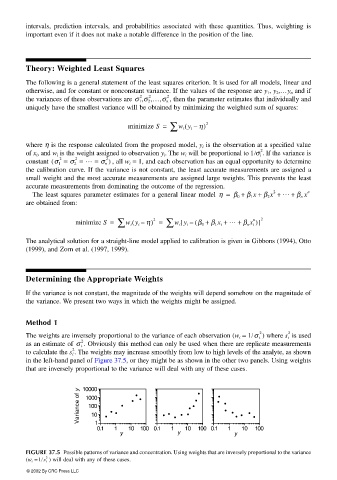
to calculate the . The weights may increase smoothly from low to high levels of the analyte, as shown
s i
in the left-hand panel of Figure 37.5, or they might be as shown in the other two panels. Using weights
that are inversely proportional to the variance will deal with any of these cases.
Variance of y 10000 • • • • • • • • • • • • • • • • • • • • • • • •
1000
100
10
1
0.1 1 10 100 0.1 1 • 10 100 0.1 1 10 100
y y y

FIGURE 37.5 Possible patterns of variance and concentration. Using weights that are inversely proportional to the variance
2
(w i = 1/s i ) will deal with any of these cases.
© 2002 By CRC Press LLC