Page 323 - Statistics for Environmental Engineers

L1592_frame_C37.fm Page 332 Tuesday, December 18, 2001 3:20 PM

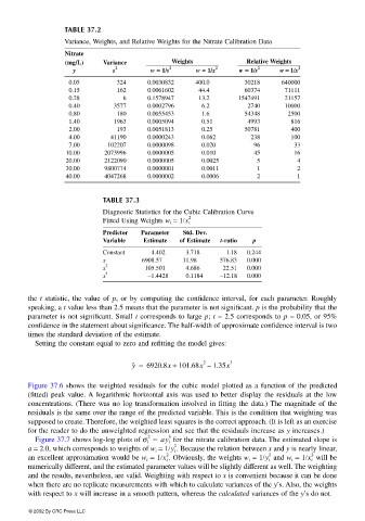
TABLE 37.2
Variance, Weights, and Relative Weights for the Nitrate Calibration Data
Nitrate
(mg/L) Variance Weights Relative Weights
2 2 2 2 2
y s w == == 1/s w == == 1/x w == == 1/s w == == 1/x
0.05 324 0.0030832 400.0 30218 640000
0.15 162 0.0061602 44.4 60374 71111
0.28 6 0.1578947 13.2 1547491 21157
0.40 3577 0.0002796 6.2 2740 10000
0.80 180 0.0055453 1.6 54348 2500
1.40 1963 0.0005094 0.51 4993 816
2.00 193 0.0051813 0.25 50781 400
4.00 41190 0.0000243 0.062 238 100
7.00 102207 0.0000098 0.020 96 33
10.00 2073996 0.0000005 0.010 45 16
20.00 2122090 0.0000005 0.0025 5 4
30.00 9800774 0.0000001 0.0011 1 2
40.00 4047268 0.0000002 0.0006 2 1

TABLE 37.3
Diagnostic Statistics for the Cubic Calibration Curve
2
Fitted Using Weights w i = 1/s i
Predictor Parameter Std. Dev.
Variable Estimate of Estimate t-ratio p
Constant 4.402 3.718 1.18 0.244
x 6908.57 11.98 576.83 0.000
2
x 105.501 4.686 22.51 0.000
3
x −1.4428 0.1184 −12.18 0.000
the t statistic, the value of p, or by computing the confidence interval, for each parameter. Roughly
speaking, a t value less than 2.5 means that the parameter is not significant. p is the probability that the
parameter is not significant. Small t corresponds to large p; t = 2.5 corresponds to p = 0.05, or 95%
confidence in the statement about significance. The half-width of approximate confidence interval is two
times the standard deviation of the estimate.
Setting the constant equal to zero and refitting the model gives:

y ˆ = 6920.8x + 101.68x – 1.35x 3
2

Figure 37.6 shows the weighted residuals for the cubic model plotted as a function of the predicted
(fitted) peak value. A logarithmic horizontal axis was used to better display the residuals at the low
concentrations. (There was no log transformation involved in fitting the data.) The magnitude of the
residuals is the same over the range of the predicted variable. This is the condition that weighting was
supposed to create. Therefore, the weighted least squares is the correct approach. (It is left as an exercise
for the reader to do the unweighted regression and see that the residuals increase as y increases.)
Figure 37.7 shows log-log plots of σ i = ay i b for the nitrate calibration data. The estimated slope is
2
2
a = 2.0, which corresponds to weights of w i = 1/ . Because the relation between x and y is nearly linear,
y i
2 2 2
an excellent approximation would be w i = 1/ . Obviously, the weights w i = 1/ and w i = 1/ will bex i y i x i
numerically different, and the estimated parameter values will be slightly different as well. The weighting
and the results, nevertheless, are valid. Weighting with respect to x is convenient because it can be done
when there are no replicate measurements with which to calculate variances of the y’s. Also, the weights
with respect to x will increase in a smooth pattern, whereas the calculated variances of the y’s do not.
© 2002 By CRC Press LLC