Page 325 - Statistics for Environmental Engineers

L1592_frame_C37.fm Page 334 Tuesday, December 18, 2001 3:20 PM

200

Frequency 100

0
0 25 50 75 100 125 150
Simulated Sample Variance, s 2

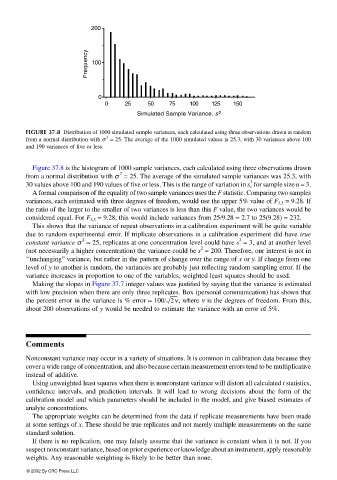
FIGURE 37.8 Distribution of 1000 simulated sample variances, each calculated using three observations drawn at random
2
from a normal distribution with σ = 25. The average of the 1000 simulated values is 25.3, with 30 variances above 100
and 190 variances of five or less.

Figure 37.8 is the histogram of 1000 sample variances, each calculated using three observations drawn
2
from a normal distribution with σ = 25. The average of the simulated sample variances was 25.3, with
2
30 values above 100 and 190 values of five or less. This is the range of variation in for sample size n = 3.
s i
A formal comparison of the equality of two sample variances uses the F statistic. Comparing two samples
variances, each estimated with three degrees of freedom, would use the upper 5% value of F 3,3 = 9.28. If
the ratio of the larger to the smaller of two variances is less than this F value, the two variances would be
considered equal. For F 3,3 = 9.28, this would include variances from 25/9.28 = 2.7 to 25(9.28) = 232.
This shows that the variance of repeat observations in a calibration experiment will be quite variable
due to random experimental error. If triplicate observations in a calibration experiment did have true
2 2
constant variance σ = 25, replicates at one concentration level could have s = 3, and at another level
2
(not necessarily a higher concentration) the variance could be s = 200. Therefore, our interest is not in
‘‘unchanging” variance, but rather in the pattern of change over the range of x or y. If change from one
level of y to another is random, the variances are probably just reflecting random sampling error. If the
variance increases in proportion to one of the variables, weighted least squares should be used.
Making the slopes in Figure 37.7 integer values was justified by saying that the variance is estimated
with low precision when there are only three replicates. Box (personal communication) has shown that
the percent error in the variance is % error = 100/ 2ν , where ν is the degrees of freedom. From this,
about 200 observations of y would be needed to estimate the variance with an error of 5%.

Comments

Nonconstant variance may occur in a variety of situations. It is common in calibration data because they
cover a wide range of concentration, and also because certain measurement errors tend to be multiplicative
instead of additive.
Using unweighted least squares when there is nonconstant variance will distort all calculated t statistics,
confidence intervals, and prediction intervals. It will lead to wrong decisions about the form of the
calibration model and which parameters should be included in the model, and give biased estimates of
analyte concentrations.
The appropriate weights can be determined from the data if replicate measurements have been made
at some settings of x. These should be true replicates and not merely multiple measurements on the same
standard solution.
If there is no replication, one may falsely assume that the variance is constant when it is not. If you
suspect nonconstant variance, based on prior experience or knowledge about an instrument, apply reasonable
weights. Any reasonable weighting is likely to be better than none.
© 2002 By CRC Press LLC