Page 326 - Statistics for Environmental Engineers

L1592_frame_C37.fm Page 335 Tuesday, December 18, 2001 3:20 PM

One reason analysts often make many measurements at low concentrations is to use the calibration
data to calculate the limit of detection for the measurement process. If this is to be done, proper weighting
is critical (Zorn et al., 1997 and 1999).

References
Currie, L. A. (1984). “Chemometrics and Analytical Chemistry,” in Chemometrics: Mathematics and Statistics
in Chemistry, NATO ASI Series C, 138, 115–146.
Danzer, K. and L. A. Currie (1998). “Guidelines for Calibration in Analytical Chemistry,” Pure Appl. Chem.,
70, 993–1014.
Gibbons, R. D. (1994). Statistical Methods for Groundwater Monitoring, New York, John Wiley.
Draper, N. R. and H. Smith, (1998). Applied Regression Analysis, 3rd ed., New York, John Wiley.
Otto, M. (1999). Chemometrics, Weinheim, Germany, Wiley-VCH.
Zorn, M. E., R. D. Gibbons, and W. C. Sonzogni (1999). ‘‘Evaluation of Approximate Methods for Calculating
the Limit of Detection and Limit of Quantitation,” Envir. Sci. & Tech., 33(13), 2291–2295.
Zorn, M. E., R. D. Gibbons, and W. C. Sonzogni (1997). “Weighted Least Squares Approach to Calculating
Limits of Detection and Quantification by Modeling Variability as a Function of Concentration,” Anal.
Chem., 69(15), 3069–3075.

Exercises
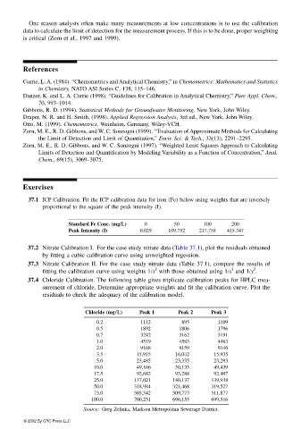
37.1 ICP Calibration. Fit the ICP calibration data for iron (Fe) below using weights that are inversely
proportional to the square of the peak intensity (I).

Standard Fe Conc. (mg/L) 0 50 100 200
Peak Intensity (I) 0.029 109.752 217.758 415.347

37.2 Nitrate Calibration I. For the case study nitrate data (Table 37.1), plot the residuals obtained
by fitting a cubic calibration curve using unweighted regession.
37.3 Nitrate Calibration II. For the case study nitrate data (Table 37.1), compare the results of
2
2
2
fitting the calibration curve using weights 1/x with those obtained using 1/s and 1/y .
37.4 Chloride Calibration. The following table gives triplicate calibration peaks for HPLC mea-
surement of chloride. Determine appropriate weights and fit the calibration curve. Plot the
residuals to check the adequacy of the calibration model.
Chloride (mg/L) Peak 1 Peak 2 Peak 3
0.2 1112 895 1109
0.5 1892 1806 1796
0.7 3242 3162 3191
1.0 4519 4583 4483
2.0 9168 9159 9146
3.5 15,915 16,042 15,935
5.0 23,485 23,335 23,293
10.0 49,166 50,135 49,439
17.5 92,682 93,288 92,407
25.0 137,021 140,137 139,938
50.0 318,984 321,468 319,527
75.0 505,542 509,773 511,877
100.0 700,231 696,155 699,516
Source: Greg Zelinka, Madison Metropolitan Sewerage District.
© 2002 By CRC Press LLC