Page 330 - Statistics for Environmental Engineers

L1592_frame_C38 Page 339 Tuesday, December 18, 2001 3:21 PM

The minimum sum of squares is called the residual sum of squares, RSS. The residual mean square
(RMS) is the residual sum of squares divided by its degrees of freedom. RMS = RSS /(n − p), where n =
number of observations and p = number of parameters estimated.

Case Study: Solution

A column settling test was done on a suspension with initial concentration of 560 mg/L. Samples were
taken at depths of 2, 4, and 6 ft (measured from the water surface) at times 20, 40, 60, and 120 min;
the data are in Table 38.1. The simplest possible model is:

C(z, t) = β 0 + β 1 t
The most complicated model that might be needed is a full quadratic function of time and depth:

2 2
C(z, t) = β 0 + β 1 t + β 2 t + β 3 z + β 4 z + β 5 zt
We can start the model building process with either of these and add or drop terms as needed.
Fitting the simplest possible model involving time and depth gives:
y ˆ = 132.3 + 7.12z 0.97t
–
2
2
which has R = 0.844 and residual mean square = 355.82. R , the coefficient of determination, is the
percentage of the total variation in the data that is accounted for by fitting the model (Chapter 39).
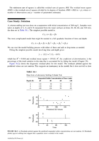
Figure 38.2a shows the diagnostic residual plots for the model. The residuals plotted against the
predicted values are not random. This suggests an inadequacy in the model, but it does not tell us how

TABLE 38.1
Data from a Laboratory Settling Column Test
Suspended Solids Concentration at Time t (min)
Depth (ft) 20 40 60 120
2 135 90 75 48
4 170 110 90 53
6 180 126 96 60

FIGURE 38.2 (a) Residuals plotted against the predicted suspended solids concentrations are not random. (b) Residuals
plotted against settling time suggest that a quadratic term is needed in the model.

© 2002 By CRC Press LLC