Page 332 - Statistics for Environmental Engineers

L1592_frame_C38 Page 341 Tuesday, December 18, 2001 3:21 PM

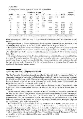
TABLE 38.3
Summary of All Possible Regressions for the Settling Test Model
Coefficient of the Term Decrease
2 2 2
Model b 0 b 1 z b 2 t b 3 z b 4 t b 5 tz R RegSS in RegSS
A 152 20.9 −2.74 −1.13 0.014 −0.08 0.985 20256
(t ratio) (2.3) (8.3) (1.0) (7.0) (2.4)
[SE] [9.1] [0.33] [1.1] [0.002] [0.03]
B 167 11.9 −2.74 0.014 −0.08 0.982 20202 54
C 171 16.1 −3.06 −1.13 0.014 0.971 19966 289
D 186 7.1 −3.06 0.143 0.968 19912 343
E 98 20.9 −0.65 −1.13 −0.08 0.864 17705 2550
F 113 11.9 −0.65 −0.08 0.858 17651 2605
G 117 16.1 −0.97 −1.13 0.849 17416 2840
H 132 7.1 −0.97 0.844 17362 2894
Note: () indicates t ratios of the estimated parameters. [] indicates standard errors of the estimated parameters.
residual mean square (RMS = 308.8/6 = 51.5) are the key statistics in comparing this model with simpler
models.
The regression sum of squares (RegSS) shows how much of the total variation (i.e., how much of the
Total SS) has been explained by the fitted equation. For this model, RegSS = 20,255.5.
2
The coefficient of determination, commonly denoted as R , is the regression sum of squares expressed
as a fraction of the total sum of squares. For the complete six-parameter model (Model A in Table 38.3),
2
R = (20256/20564) = 0.985, so it can be said that this model accounts for 98.5% of the total variation
in the data.
2
It is natural to be fascinated by high R values and this tempts us to think that the goal of model building
2
is to make R as high as possible. Obviously, this can be done by putting more high-order terms into a
model, but it should be equally obvious that this does not necessarily improve the predictions that will
2
2
be made using the model. Increasing R is the wrong goal. Instead of worrying about R values, we
should seek the simplest adequate model.
Selecting the “Best” Regression Model

The “best” model is the one that adequately describes the data with the fewest parameters. Table 38.3
2
summarizes parameter estimates, the coefficient of determination R , and the regression sum of squares
for all eight possible linear models. The total sum of squares, of course, is the same in all eight cases
because it depends on the data and not on the form of the model. Standard errors [SE] and t ratios (in
parentheses) are given for the complete model, Model A.
One approach is to examine the t ratio for each parameter. Roughly speaking, if a parameter’s t ratio
is less than 2.5, the true value of the parameter could be zero and that term could be dropped from the
equation.
Another approach is to examine the confidence intervals of the estimated parameters. If this interval
includes zero, the variable associated with the parameter can be dropped from the model. For example,
2
in Model A, the coefficient of z is b 3 = −1.13 with standard error = 1.1 and 95% confidence interval
[ −3.88 to +1.62]. This confidence interval includes zero, indicating that the true value of b 3 is very likely
2
to be zero, and therefore the term z can be tentatively dropped from the model. Fitting the simplified
2
model (without z ) gives Model B in Table 38.3.
The standard error [SE] is the number in brackets. The half-width of the 95% confidence interval is
a multiple of the standard error of the estimated value. The multiplier is a t statistic that depends on the
selected level of confidence and the degrees of freedom. This multiplier is not the same value as the
t ratio given in Table 38.3. Roughly speaking, if the degrees of freedom are large (n − p ≥ 20), the half-
width of the confidence interval is about 2SE for a 95% confidence interval. If the degrees of freedom
are small (n − p < 10), the multiplier will be in the range of 2.3SE to 3.0SE.
© 2002 By CRC Press LLC