Page 337 - Statistics for Environmental Engineers

L1592_frame_C39 Page 346 Tuesday, December 18, 2001 3:22 PM

2 2
This shows that R is a model comparison and that large R measures only how much the model improves
the null model. It does not indicate how good the model is in any absolute sense. Consequently, the
2
common belief that a large R demonstrates model adequacy is sometimes wrong.
2
The definition of R also shows that comparisons are made only between nested models. The concept
of proportionate reduction in variation is untrustworthy unless one model is a special case of the other.
2
This means that R cannot be used to compare models with an intercept with models that have no
intercept: y = β 0 is not a reduction of the model y = β 1 x. It is a reduction of y = β 0 + β 1 x and y = β 0 +
2
β 1 x + β 2 x .

2
A High R Does Not Assure a Valid Relation
2
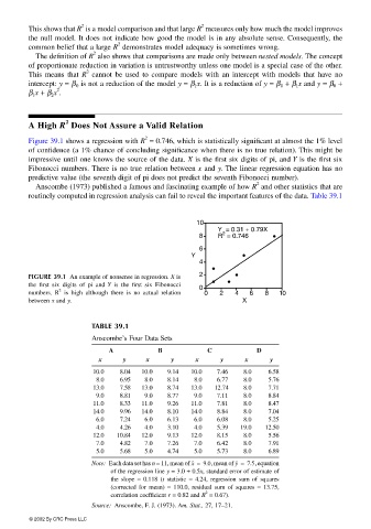
Figure 39.1 shows a regression with R = 0.746, which is statistically significant at almost the 1% level
of confidence (a 1% chance of concluding significance when there is no true relation). This might be
impressive until one knows the source of the data. X is the first six digits of pi, and Y is the first six
Fibonocci numbers. There is no true relation between x and y. The linear regression equation has no
predictive value (the seventh digit of pi does not predict the seventh Fibonocci number).
2
Anscombe (1973) published a famous and fascinating example of how R and other statistics that are
routinely computed in regression analysis can fail to reveal the important features of the data. Table 39.1

10
Y = 0.31 + 0.79X
2
8 R = 0.746
6
Y
4
FIGURE 39.1 An example of nonsense in regression. X is 2
the first six digits of pi and Y is the first six Fibonocci 0
2
numbers. R is high although there is no actual relation 0 2 4 6 8 10
between x and y. X

TABLE 39.1
Anscombe’s Four Data Sets
A B C D
x y x y x y x y
10.0 8.04 10.0 9.14 10.0 7.46 8.0 6.58
8.0 6.95 8.0 8.14 8.0 6.77 8.0 5.76
13.0 7.58 13.0 8.74 13.0 12.74 8.0 7.71
9.0 8.81 9.0 8.77 9.0 7.11 8.0 8.84
11.0 8.33 11.0 9.26 11.0 7.81 8.0 8.47
14.0 9.96 14.0 8.10 14.0 8.84 8.0 7.04
6.0 7.24 6.0 6.13 6.0 6.08 8.0 5.25
4.0 4.26 4.0 3.10 4.0 5.39 19.0 12.50
12.0 10.84 12.0 9.13 12.0 8.15 8.0 5.56
7.0 4.82 7.0 7.26 7.0 6.42 8.0 7.91
5.0 5.68 5.0 4.74 5.0 5.73 8.0 6.89
Note: Each data set has n = 11, mean of x = 9.0, mean of y = 7.5, equation
of the regression line y = 3.0 + 0.5x, standard error of estimate of
the slope = 0.118 (t statistic = 4.24, regression sum of squares
(corrected for mean) = 110.0, residual sum of squares = 13.75,
2
correlation coefficient r = 0.82 and R = 0.67).
Source: Anscombe, F. J. (1973). Am. Stat., 27, 17–21.
© 2002 By CRC Press LLC