Page 340 - Statistics for Environmental Engineers

L1592_frame_C39 Page 349 Tuesday, December 18, 2001 3:22 PM

30
R 2 = 0.77 R 2 = 0.12
• •
• • • •
• • • • • • • • •
•
•
y 20 • • • • • • • • • • • • • • •
•
• •
• •
• • • • • • • •
• • • • • •
•
• • • •
• •
• •
• •
10
30 •
R 2 = 0.88 R 2 = 0.93
• •
• • • •
• • • •
y 20 • •
•
• •
• •
• •
• •
10
10 15 20 10 15 20
x x
2 2
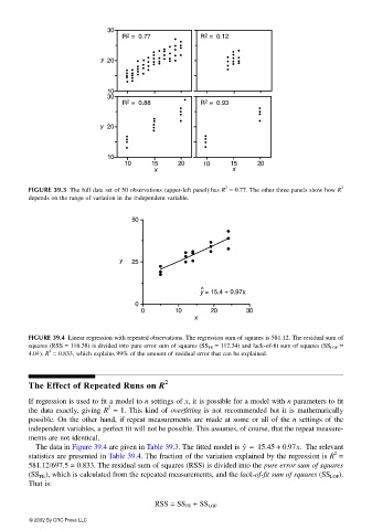
FIGURE 39.3 The full data set of 50 observations (upper-left panel) has R = 0.77. The other three panels show how R
depends on the range of variation in the independent variable.
50
y 25

^
y = 15.4 + 0.97x
0
0 10 20 30
x

FIGURE 39.4 Linear regression with repeated observations. The regression sum of squares is 581.12. The residual sum of
squares (RSS = 116.38) is divided into pure error sum of squares (SS PE = 112.34) and lack-of-fit sum of squares (SS LOF =
2
4.04). R = 0.833, which explains 99% of the amount of residual error that can be explained.

The Effect of Repeated Runs on R 2

If regression is used to fit a model to n settings of x, it is possible for a model with n parameters to fit
2
the data exactly, giving R = 1. This kind of overfitting is not recommended but it is mathematically
possible. On the other hand, if repeat measurements are made at some or all of the n settings of the
independent variables, a perfect fit will not be possible. This assumes, of course, that the repeat measure-
ments are not identical.
The data in Figure 39.4 are given in Table 39.3. The fitted model is y ˆ = 15.45 + 0.97x. The relevant
statistics are presented in Table 39.4. The fraction of the variation explained by the regression is R =
2
581.12/697.5 = 0.833. The residual sum of squares (RSS) is divided into the pure error sum of squares
(SS PE ), which is calculated from the repeated measurements, and the lack-of-fit sum of squares (SS LOF ).
That is:

RSS = SS PE + SS LOF
© 2002 By CRC Press LLC