Page 343 - Statistics for Environmental Engineers

L1592_frame_C39 Page 352 Tuesday, December 18, 2001 3:22 PM

2
Totally spurious correlations, often with high R values, can arise when unrelated variables are
combined. Two examples of particular interest to environmental engineers are presented by Sherwood
(1974) and Rowe (1974). Both emphasize graphical analysis to stimulate and support any regression
analysis. Rowe discusses the particular dangers that arise when sets of variables are combined to create
new variables such as dimensional numbers (Froude number, etc.). Benson (1965) points out the same
kinds of dangers in the context of hydraulics and hydrology.

References
2
Anderson-Sprecher, R. (1994). “Model Comparison and R ,” Am. Stat., 48(2), 113–116.
Anscombe, F. J. (1973). “Graphs in Statistical Analysis,” Am. Stat., 27, 17–21.
Benson, M. A. (1965). “Spurious Correlation in Hydraulics and Hydrology,” J. Hydraulics Div., ASCE, 91,
HY4, 35–45.
Box, G. E. P. (1966). “The Use and Abuse of Regression,” Technometrics, 8, 625–629.
Box, G. E. P. and J. Wetz (1973). “Criteria for Judging Accuracy of Estimation by an Approximating Response
Function,” Madison, WI, University of Wisconsin Statistics Department, Tech. Rep. No. 9.
Draper, N. R. and H. Smith (1998). Applied Regression Analysis, 3rd ed., New York, John Wiley.
Hahn, G. J. (1973). “The Coefficient of Determination Exposed,” Chemtech, October, pp. 609–611.
Rowe, P. N. (1974). “Correlating Data,” Chemtech, January, pp. 9–14.
Sherwood, T. K. (1974). “The Treatment and Mistreatment of Data,” Chemtech, December, pp. 736–738.
Tufte, E. R. (1983). The Visual Display of Quantitative Information, Cheshire, CT, Graphics Press.

Exercises
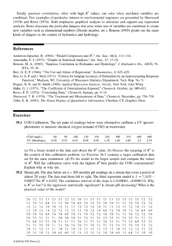
39.1 COD Calibration. The ten pairs of readings below were obtained to calibrate a UV spectro-
photometer to measure chemical oxygen demand (COD) in wastewater.

COD (mg/L) 60 90 100 130 195 250 300 375 500 600
UV Absorbance 0.30 0.35 0.45 0.48 0.95 1.30 1.60 1.80 2.3 2.55

2
2
(a) Fit a linear model to the data and obtain the R value. (b) Discuss the meaning of R in
the context of this calibration problem. (c) Exercise 36.3 contains a larger calibration data
set for the same instrument. (d) Fit the model to the larger sample and compare the values
2
2
of R . Will the calibration curve with the highest R best predict the COD concentration?
Explain why or why not.
39.2 Stream pH. The data below are n = 200 monthly pH readings on a stream that cover a period of
almost 20 years. The data read from left to right. The fitted regression model is = 7.1435 −
y ˆ
2
0.0003776t; R = 0.042. The confidence interval of the slope is [−0.00063, −0.000013]. Why
2
is R so low? Is the regression statistically significant? Is stream pH decreasing? What is the
practical value of the model?
7.0 7.2 7.2 7.3 7.2 7.2 7.2 7.2 7.0 7.1 7.3 7.1 7.1 7.1 7.2 7.3 7.2 7.3 7.2 7.2
7.1 7.4 7.1 6.8 7.3 7.3 7.0 7.0 6.9 7.2 7.2 7.3 7.0 7.0 7.1 7.1 7.0 7.2 7.2 7.2
7.2 7.1 7.2 7.0 7.0 7.2 7.1 7.1 7.2 7.2 7.2 7.0 7.1 7.1 7.2 7.1 7.2 7.0 7.1 7.2
7.1 7.0 7.1 7.4 7.2 7.2 7.2 7.2 7.1 7.0 7.2 7.0 6.9 7.2 7.0 7.0 7.1 7.0 6.9 6.9
7.0 7.0 7.2 6.9 7.4 7.0 6.9 7.0 7.1 7.0 7.2 7.2 7.0 7.0 7.1 7.1 7.0 7.2 7.2 7.0
7.0 7.2 7.1 7.1 7.1 7.0 7.0 7.0 7.1 7.3 7.1 7.2 7.2 7.2 7.1 7.2 7.2 7.1 7.1 7.1
7.2 6.8 7.2 7.2 7.0 7.1 7.1 7.2 7.0 7.1 7.1 7.1 7.0 7.2 7.1 7.1 7.3 6.9 7.2 7.2
7.1 7.1 7.0 7.0 7.1 7.1 7.0 7.0 7.0 7.1 7.0 7.1 7.1 7.2 7.2 7.1 7.0 7.0 7.2 7.2
7.0 7.1 7.2 7.1 7.1 7.0 7.1 7.0 7.2 7.1 7.1 7.1 7.2 7.1 7.0 7.1 7.2 7.2 7.1 7.2
7.0 7.1 7.0 7.1 7.0 6.9 6.9 7.2 7.1 7.2 7.1 7.1 7.0 7.0 6.9 7.1 6.8 7.1 7.0 7.0

© 2002 By CRC Press LLC