Page 346 - Statistics for Environmental Engineers

L1592_frame_C40 Page 356 Tuesday, December 18, 2001 3:24 PM

7.0

6.5
pH
6.0

5.5
0 100 200 300 400 500 600 700
Weak Acidity (µg/L)

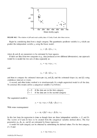
FIGURE 40.1 The relation of pH and weak acidity data of Cosby Creek after three storms.

Begin by considering data from a single category. The quantitative predictor variable is x 1 which can
predict the independent variable y 1 using the linear model:

y 1i = β 0 + β 1 x 1i + e i

where β 0 and β 1 are parameters to be estimated by least squares.
If there are data from two categories (e.g., data produced at two different laboratories), one approach
would be to model the two sets of data separately as:
y 1i = α 0 + α 1 x 1i + e i

and
y 2i = β 0 + β 1 x 2i + e i

and then to compare the estimated intercepts (α 0 and β 0 ) and the estimated slopes (α 1 and β 1 ) using
confidence intervals or t-tests.
A second, and often better, method is to simultaneously fit a single augmented model to all the data.
To construct this model, define a categorical variable Z as follows:

Z = 0 if the data are in the first category
Z = 1 if the data are in the second category

The augmented model is:
y i = α 0 + α 1 x i + Z β 0 + β 1 x i ) + e i
(
With some rearrangement:

y i = α 0 + β 0 Z + α 1 x i + β 1 Zx i + e i

In this last form the regression is done as though there are three independent variables, x, Z, and Zx.
The vectors of Z and Zx have to be created from the categorical variables defined above. The four
parameters α 0 , β 0 , α 1 , and β 1 are estimated by linear regression.
A model for each category can be obtained by substituting the defined values. For the first category,
Z = 0 and:

y i = α 0 + α 1 x i + e i
© 2002 By CRC Press LLC