Page 350 - Statistics for Environmental Engineers

L1592_frame_C40 Page 360 Tuesday, December 18, 2001 3:24 PM

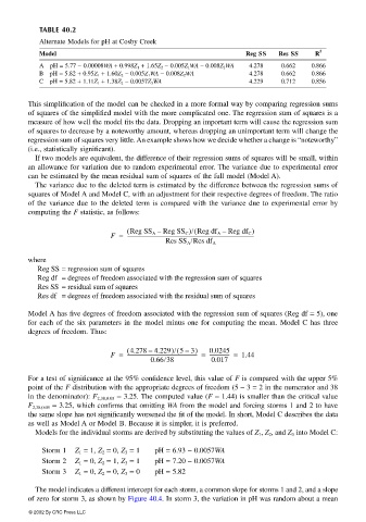
TABLE 40.2
Alternate Models for pH at Cosby Creek
Model Reg SS Res SS R 2
A pH = 5.77 − 0.00008WA + 0.998Z 1 + 1.65Z 2 − 0.005Z 1 WA − 0.008Z 2 WA 4.278 0.662 0.866
B pH = 5.82 + 0.95Z 1 + 1.60Z 2 − 0.005Z 1 WA − 0.008Z 2 WA 4.278 0.662 0.866
C pH = 5.82 + 1.11Z 1 + 1.38Z 2 − 0.0057Z 3 WA 4.229 0.712 0.856

This simplification of the model can be checked in a more formal way by comparing regression sums
of squares of the simplified model with the more complicated one. The regression sum of squares is a
measure of how well the model fits the data. Dropping an important term will cause the regression sum
of squares to decrease by a noteworthy amount, whereas dropping an unimportant term will change the
regression sum of squares very little. An example shows how we decide whether a change is “noteworthy”
(i.e., statistically significant).
If two models are equivalent, the difference of their regression sums of squares will be small, within
an allowance for variation due to random experimental error. The variance due to experimental error
can be estimated by the mean residual sum of squares of the full model (Model A).
The variance due to the deleted term is estimated by the difference between the regression sums of
squares of Model A and Model C, with an adjustment for their respective degrees of freedom. The ratio
of the variance due to the deleted term is compared with the variance due to experimental error by
computing the F statistic, as follows:

(
( Reg SS A – Reg SS C )/ Reg df A – Reg df C )
F = ------------------------------------------------------------------------------------------------------
Res SS A /Res df A
where
Reg SS = regression sum of squares
Reg df = degrees of freedom associated with the regression sum of squares
Res SS = residual sum of squares
Res df = degrees of freedom associated with the residual sum of squares
Model A has five degrees of freedom associated with the regression sum of squares (Reg df = 5), one
for each of the six parameters in the model minus one for computing the mean. Model C has three
degrees of freedom. Thus:

(
( 4.278 4.229)/ 53) 0.0245
–
–
F = --------------------------------------------------------- = ---------------- = 1.44
0.66/38 0.017
For a test of significance at the 95% confidence level, this value of F is compared with the upper 5%
point of the F distribution with the appropriate degrees of freedom (5 – 3 = 2 in the numerator and 38
in the denominator): F 2,38,0.05 = 3.25. The computed value (F = 1.44) is smaller than the critical value
F 2,38,0.05 = 3.25, which confirms that omitting WA from the model and forcing storms 1 and 2 to have
the same slope has not significantly worsened the fit of the model. In short, Model C describes the data
as well as Model A or Model B. Because it is simpler, it is preferred.
Models for the individual storms are derived by substituting the values of Z 1 , Z 2 , and Z 3 into Model C:
Storm 1 Z 1 = 1, Z 2 = 0, Z 3 = 1 pH = 6.93 − 0.0057WA
Storm 2 Z 1 = 0, Z 2 = 1, Z 3 = 1 pH = 7.20 − 0.0057WA
Storm 3 Z 1 = 0, Z 2 = 0, Z 3 = 0 pH = 5.82

The model indicates a different intercept for each storm, a common slope for storms 1 and 2, and a slope
of zero for storm 3, as shown by Figure 40.4. In storm 3, the variation in pH was random about a mean
© 2002 By CRC Press LLC