Page 348 - Statistics for Environmental Engineers

L1592_frame_C40 Page 358 Tuesday, December 18, 2001 3:24 PM

estimate β 0 = 0, γ 0 = 0, β 1 = 0, and γ 1 = 0 and the same slope (α 1 ) and intercept (α 0 ) would apply to

all three categories. The fitted simplified model is y i = α 0 + α 1 x i + e i .
If the intercepts are different for the three categories but the slopes are the same, the regression would
estimate β 1 = 0 and γ 1 = 0 and the model becomes:
y i = ( α 0 + β 0 Z 1 + γ 0 Z 2 ) + α 1 x i + e i

For category 1: y i = ( α 0 + β 0 Z 1 ) + α 1 x i + e i
For category 2: y i = ( α 0 + γ 0 Z 2 ) + α 1 x i + e i
For category 3: y i = α 0 + α 1 x i + e i

Case Study: Solution
The model under consideration allows a different slope and intercept for each storm. Two dummy variables
are needed:

Z 1 = 1 for storm 1 and zero otherwise
Z 2 = 1 for storm 2 and zero otherwise

The model is:

pH = α 0 + α 1 WA + Z 1 (β 0 + β 1 WA ) + Z 2 (γ 0 + γ 1 WA )

where the α’s, β’s, and γ ’s are estimated by regression. The model can be rewritten as:

pH = α 0 + β 0 Z 1 + γ 0 Z 2 + α 1 WA + β 1 Z 1 WA + γ 1 Z 2 WA

The dummy variables are incorporated into the model by creating the new variables Z 1 WA and Z 2 WA.
Table 40.1 shows how this is done.
Fitting the full six-parameter model gives:

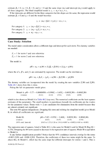
Model A: pH = 5.77 − 0.00008WA + 0.998Z 1 + 1.65Z 2 − 0.005Z 1 WA − 0.008Z 2 WA
(t-ratios) (0.11) (2.14) (3.51) (3.63) (4.90)

which is also shown as Model A in Table 40.2 (top row). The numerical coefficients are the least squares
estimates of the parameters. The small numbers in parentheses beneath the coefficients are the t-ratios
for the parameter values. Terms with t < 2 are candidates for elimination from the model because they
are almost certainly not significant.
The term WA appears insignificant. Dropping this term and refitting the simplified model gives Model
B, in which all coefficients are significant:

Model B: pH = 5.82 + 0.95Z 1 + 1.60Z 2 − 0.005Z 1 WA − 0.008Z 2 WA
(t-ratios) (6.01) (9.47) (4.35) (5.54)
[95% conf. interval] [0.63 to 1.27] [1.26 to 1.94] [−0.007 to −0.002] [−0.01 to −0.005]
The regression sum of squares, listed in Table 40.2, is the same for Model A and for Model B (Reg SS =
4.278). Dropping the WA term caused no decrease in the regression sum of squares. Model B is equivalent
to Model A.
Is any further simplification possible? Notice that the 95% confidence intervals overlap for the terms
−0.005 Z 1 WA and –0.008 Z 2 WA. Therefore, the coefficients of these two terms might be the same. To
check this, fit Model C, which has the same slope but different intercepts for storms 1 and 2. This is
© 2002 By CRC Press LLC