Page 351 - Statistics for Environmental Engineers

L1592_frame_C40 Page 361 Tuesday, December 18, 2001 3:24 PM

7.0

pH = 7.20 - 0.0057 WA
6.5
pH

6.0
pH = 5.82
pH = 6.93 - 0.0057 WA
5.5
0 100 200 300 400 500 600 700
Weak Acidity (mg/L)

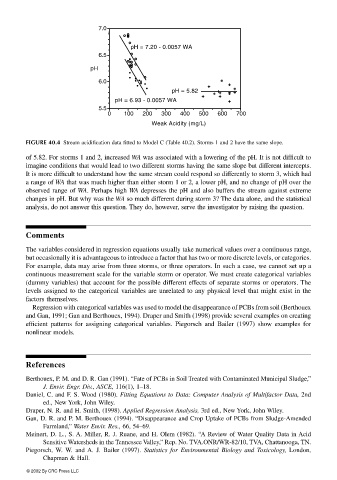
FIGURE 40.4 Stream acidification data fitted to Model C (Table 40.2). Storms 1 and 2 have the same slope.

of 5.82. For storms 1 and 2, increased WA was associated with a lowering of the pH. It is not difficult to
imagine conditions that would lead to two different storms having the same slope but different intercepts.
It is more difficult to understand how the same stream could respond so differently to storm 3, which had
a range of WA that was much higher than either storm 1 or 2, a lower pH, and no change of pH over the
observed range of WA. Perhaps high WA depresses the pH and also buffers the stream against extreme
changes in pH. But why was the WA so much different during storm 3? The data alone, and the statistical
analysis, do not answer this question. They do, however, serve the investigator by raising the question.

Comments

The variables considered in regression equations usually take numerical values over a continuous range,
but occasionally it is advantageous to introduce a factor that has two or more discrete levels, or categories.
For example, data may arise from three storms, or three operators. In such a case, we cannot set up a
continuous measurement scale for the variable storm or operator. We must create categorical variables
(dummy variables) that account for the possible different effects of separate storms or operators. The
levels assigned to the categorical variables are unrelated to any physical level that might exist in the
factors themselves.
Regression with categorical variables was used to model the disappearance of PCBs from soil (Berthouex
and Gan, 1991; Gan and Berthouex, 1994). Draper and Smith (1998) provide several examples on creating
efficient patterns for assigning categorical variables. Piegorsch and Bailer (1997) show examples for
nonlinear models.

References
Berthouex, P. M. and D. R. Gan (1991). “Fate of PCBs in Soil Treated with Contaminated Municipal Sludge,”
J. Envir. Engr. Div., ASCE, 116(1), 1–18.
Daniel, C. and F. S. Wood (1980). Fitting Equations to Data: Computer Analysis of Multifactor Data, 2nd
ed., New York, John Wiley.
Draper, N. R. and H. Smith, (1998). Applied Regression Analysis, 3rd ed., New York, John Wiley.
Gan, D. R. and P. M. Berthouex (1994). “Disappearance and Crop Uptake of PCBs from Sludge-Amended
Farmland,” Water Envir. Res., 66, 54–69.
Meinert, D. L., S. A. Miller, R. J. Ruane, and H. Olem (1982). “A Review of Water Quality Data in Acid
Sensitive Watersheds in the Tennessee Valley,” Rep. No. TVA.ONR/WR-82/10, TVA, Chattanooga, TN.
Piegorsch, W. W. and A. J. Bailer (1997). Statistics for Environmental Biology and Toxicology, London,
Chapman & Hall.
© 2002 By CRC Press LLC