Page 338 - Statistics for Environmental Engineers

L1592_frame_C39 Page 347 Tuesday, December 18, 2001 3:22 PM

15
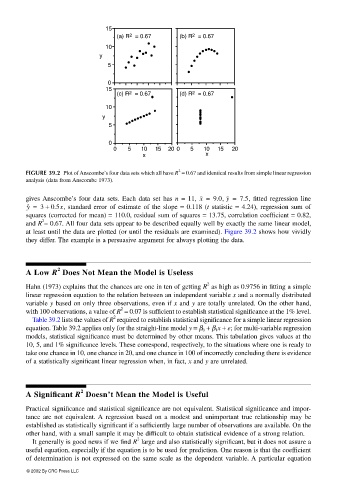
(a) R 2 = 0.67 (b) R 2 = 0.67
10
y
5

0
15
(c) R 2 = 0.67 (d) R 2 = 0.67
10
y
5

0
0 5 10 15 20 0 5 10 15 20
x x
2
FIGURE 39.2 Plot of Anscombe’s four data sets which all have R = 0.67 and identical results from simple linear regression
analysis (data from Anscombe 1973).

gives Anscombe’s four data sets. Each data set has n = 11, x = 9.0, y = 7.5, fitted regression line
y ˆ = 3 + 0.5x, standard error of estimate of the slope = 0.118 (t statistic = 4.24), regression sum of
squares (corrected for mean) = 110.0, residual sum of squares = 13.75, correlation coefficient = 0.82,
2
and R = 0.67. All four data sets appear to be described equally well by exactly the same linear model,
at least until the data are plotted (or until the residuals are examined). Figure 39.2 shows how vividly
they differ. The example is a persuasive argument for always plotting the data.

2
A Low R Does Not Mean the Model is Useless
2
Hahn (1973) explains that the chances are one in ten of getting R as high as 0.9756 in fitting a simple
linear regression equation to the relation between an independent variable x and a normally distributed
variable y based on only three observations, even if x and y are totally unrelated. On the other hand,
2
with 100 observations, a value of R = 0.07 is sufficient to establish statistical significance at the 1% level.
2
Table 39.2 lists the values of R required to establish statistical significance for a simple linear regression
equation. Table 39.2 applies only for the straight-line model y = β 0 + β 1 x + e; for multi-variable regression
models, statistical significance must be determined by other means. This tabulation gives values at the
10, 5, and 1% significance levels. These correspond, respectively, to the situations where one is ready to
take one chance in 10, one chance in 20, and one chance in 100 of incorrectly concluding there is evidence
of a statistically significant linear regression when, in fact, x and y are unrelated.

2
A Significant R Doesn’t Mean the Model is Useful
Practical significance and statistical significance are not equivalent. Statistical significance and impor-
tance are not equivalent. A regression based on a modest and unimportant true relationship may be
established as statistically significant if a sufficiently large number of observations are available. On the
other hand, with a small sample it may be difficult to obtain statistical evidence of a strong relation.
2
It generally is good news if we find R large and also statistically significant, but it does not assure a
useful equation, especially if the equation is to be used for prediction. One reason is that the coefficient
of determination is not expressed on the same scale as the dependent variable. A particular equation
© 2002 By CRC Press LLC