Page 331 - Statistics for Environmental Engineers

L1592_frame_C38 Page 340 Tuesday, December 18, 2001 3:21 PM

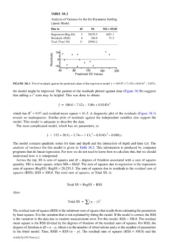
TABLE 38.2
Analysis of Variance for the Six-Parameter Settling
Linear Model
Due to df SS MS = SS/df
Regression (Reg SS) 5 20255.5 4051.1
Residuals (RSS) 6 308.8 51.5
Total (Total SS) 11 20564.2

10 • • • • •
Residuals 0 • • • • •

-10
40 80 • 120 • 160 200
Predicted SS Values

2
y ˆ
FIGURE 38.3 Plot of residuals against the predicted values of the regression model = 185.97 + 7.125t + 0.014t − 3.057z.
the model might be improved. The pattern of the residuals plotted against time (Figure 38.2b) suggests
2
that adding a t term may be helpful. This was done to obtain:
y ˆ = 186.0 + 7.12z 3.06t + 0.0143t 2
–
2
which has R = 0.97 and residual mean square = 81.5. A diagnostic plot of the residuals (Figure 38.3)
reveals no inadequacies. Similar plots of residuals against the independent variables also support the
model. This model is adequate to describe the data.
The most complicated model, which has six parameters, is:

y ˆ = 152 + 20.9z 2.74t – 1.13z – 0.0143t – 0.080zt
2
2
–
The model contains quadratic terms for time and depth and the interaction of depth and time (zt). The
analysis of variance for this model is given in Table 38.2. This information is produced by computer
programs that do linear regression. For now we do not need to know how to calculate this, but we should
understand how it is interpreted.
Across the top, SS is sum of squares and df = degrees of freedom associated with a sum of squares
quantity. MS is mean square, where MS = SS/df. The sum of squares due to regression is the regression
sum of squares (RegSS): RegSS = 20,255.5. The sum of squares due to residuals is the residual sum of
squares (RSS); RSS = 308.8. The total sum of squares, or Total SS, is:

Total SS = RegSS + RSS

Also:

Total SS = ∑ ( y i – y) 2

The residual sum of squares (RSS) is the minimum sum of squares that results from estimating the parameters
by least squares. It is the variation that is not explained by fitting the model. If the model is correct, the RSS
is the variation in the data due to random measurement error. For this model, RSS = 308.8. The residual
mean square is the RSS divided by the degrees of freedom of the residual sum of squares. For RSS, the
degrees of freedom is df = n − p, where n is the number of observations and p is the number of parameters
in the fitted model. Thus, RMS = RSS /(n − p). The residual sum of squares (RSS = 308.8) and the
© 2002 By CRC Press LLC