Page 305 - Statistics for Environmental Engineers

L1592_frame_C35 Page 312 Tuesday, December 18, 2001 2:52 PM

Approx. 95%
confidence region
0.15 200 S = 0.0058
0.001
0.002 0.002
Growth Rate (1/h) 0.15 y = 55.4 + x θ 2 100 0.007
0.007
150
0.0058
0.10
0.153x
50
0 00
0 100 200 300 0 0.1 0.2 0.3 0.4
Substrate Concentration (mg/L) θ 1

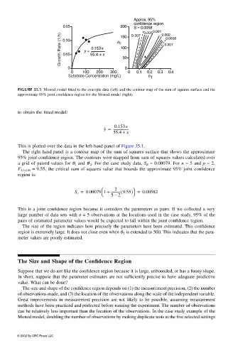
FIGURE 35.1 Monod model fitted to the example data (left) and the contour map of the sum of squares surface and the
approximate 95% joint confidence region for the Monod model (right).

to obtain the fitted model:

0.153x
y ˆ = -------------------
55.4 + x

This is plotted over the data in the left-hand panel of Figure 35.1.
The right-hand panel is a contour map of the sum of squares surface that shows the approximate
95% joint confidence region. The contours were mapped from sum of squares values calculated over
a grid of paired values for θ 1 and θ 2 . For the case study data, S R = 0.00079. For n = 5 and p = 2,
F 2,3,0.05 = 9.55, the critical sum of squares value that bounds the approximate 95% joint confidence
region is:



2
S c = 0.00079 1 + ------------ 9.55( ) = 0.00582


52
–
This is a joint confidence region because it considers the parameters as pairs. If we collected a very
large number of data sets with n = 5 observations at the locations used in the case study, 95% of the
pairs of estimated parameter values would be expected to fall within the joint confidence region.
The size of the region indicates how precisely the parameters have been estimated. This confidence
region is extremely large. It does not close even when θ 2 is extended to 500. This indicates that the para-
meter values are poorly estimated.

The Size and Shape of the Confidence Region
Suppose that we do not like the confidence region because it is large, unbounded, or has a funny shape.
In short, suppose that the parameter estimates are not sufficiently precise to have adequate predictive
value. What can be done?
The size and shape of the confidence region depends on (1) the measurement precision, (2) the number
of observations made, and (3) the location of the observations along the scale of the independent variable.
Great improvements in measurement precision are not likely to be possible, assuming measurement
methods have been practiced and perfected before running the experiment. The number of observations
can be relatively less important than the location of the observations. In the case study example of the
Monod model, doubling the number of observations by making duplicate tests at the five selected settings

© 2002 By CRC Press LLC