Page 298 - Statistics for Environmental Engineers

L1592_frame_C34 Page 304 Tuesday, December 18, 2001 2:52 PM

(a) (b)
β
2

β β
1 1
(c) (d )
θ
2

θ 1 θ 1

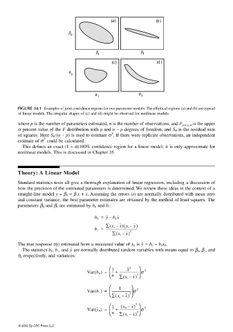
FIGURE 34.1 Examples of joint confidence regions for two parameter models. The elliptical regions (a) and (b) are typical
of linear models. The irregular shapes of (c) and (d) might be observed for nonlinear models.

where p is the number of parameters estimated, n is the number of observations, and F p,n−p,α is the upper
α percent value of the F distribution with p and n – p degrees of freedom, and S R is the residual sum
2
of squares. Here S R /(n − p) is used to estimate σ . If there were replicate observations, an independent
2
estimate of σ could be calculated.
This defines an exact (1 − α)100% confidence region for a linear model; it is only approximate for
nonlinear models. This is discussed in Chapter 35.

Theory: A Linear Model
Standard statistics texts all give a thorough explanation of linear regression, including a discussion of
how the precision of the estimated parameters is determined. We review these ideas in the context of a
straight-line model y = β 0 + β 1 x + e. Assuming the errors (e) are normally distributed with mean zero
and constant variance, the best parameter estimates are obtained by the method of least squares. The
parameters β 0 and β 1 are estimated by b 0 and b 1 :

b 0 = yb 1 x
–
(
(
∑ x i – x) y i – y)
b 1 = ----------------------------------------
∑ x i –( x) 2
The true response (η) estimated from a measured value of x 0 is = b 0 − b 1 x 0 .y ˆ
y ˆ
The statistics b 0 , b 1 , and are normally distributed random variables with means equal to β 0 , β 1 , and
η, respectively, and variances:

1  2 
x
()
Var b 0 =  --- + ------------------------σ 2
2
(
 n ∑ x i – x) 
 
1
Var b 1 =  ------------------------σ 2
()
 ∑ x i –( x) 
2
1  ( x 0 – x) 
2
Var y ˆ () =  --- + ------------------------σ 2
0
2
(
 n ∑ x i – x) 
© 2002 By CRC Press LLC