Page 290 - Statistics for Environmental Engineers

L1592_frame_C33 Page 296 Tuesday, December 18, 2001 2:51 PM

and independent variables are known. It is the parameters, the β’s and θ’s, that are unknown and must
2
2
be computed. The model y = βx is nonlinear in x; but once the known value of x is provided, we have
an equation that is linear in the parameter β. This is a linear model and it can be fitted by linear regression.
θ
In contrast, the model y = x is nonlinear in θ, and θ must be estimated by nonlinear regression (or we
must transform the model to make it linear).
It is usually assumed that a well-conducted experiment produces values of x i that are essentially
without error, while the observations of y i are affected by random error. Under this assumption, the y i
observed for the ith experimental run is the sum of the true underlying value of the response (η i ) and a
residual error (e i ):
y i = η i + e i i = 1, 2,…,n

Suppose that we know, or tentatively propose, the linear model η = β 0 + β 1 x. The observed responses
to which the model will be fitted are:

+
y i = β 0 β 1 x i + e i
which has residuals:

e i = y i β 0 β 1 x i
–
–
Similarly, if one proposed the nonlinear model η = θ 1 exp(−θ 2 x), the observed response is:

y i = θ 1 exp(−θ 2 x i ) + e i
with residuals:

e i = y i − θ 1 exp(−θ 2 x i )

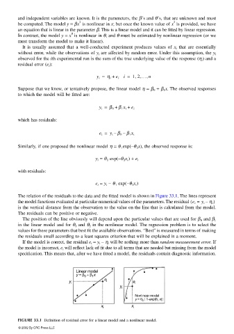
The relation of the residuals to the data and the fitted model is shown in Figure 33.1. The lines represent
the model functions evaluated at particular numerical values of the parameters. The residual e i =( y i η i )
–
is the vertical distance from the observation to the value on the line that is calculated from the model.
The residuals can be positive or negative.
The position of the line obviously will depend upon the particular values that are used for β 0 and β 1
in the linear model and for θ 1 and θ 2 in the nonlinear model. The regression problem is to select the
values for these parameters that best fit the available observations. “Best” is measured in terms of making
the residuals small according to a least squares criterion that will be explained in a moment.
If the model is correct, the residual e i = y i − η i will be nothing more than random measurement error. If
the model is incorrect, e i will reflect lack-of-fit due to all terms that are needed but missing from the model
specification. This means that, after we have fitted a model, the residuals contain diagnostic information.

Linear model
y = β + β x
1
0
e
y i i e i
y i
Nonlinear model
y = θ [ 1-exp(θ x)]
1
0
x i x i
FIGURE 33.1 Definition of residual error for a linear model and a nonlinear model.
© 2002 By CRC Press LLC