Page 286 - Statistics for Environmental Engineers

L1592_frame_C32 Page 291 Tuesday, December 18, 2001 2:50 PM

250 250

BOD t - 1 200 200 BOD t - 3
150
150
100 100
r 1 = -0.49 r 6 = -0.03
50 50
250 250
BOD t - 6 200 200 BOD t - 12

150
150
100 100
r 12 = -0.42 r 24 = -0.25
50 50
50 100 150 200 25050 100 150 200 250
BOD t BOD t
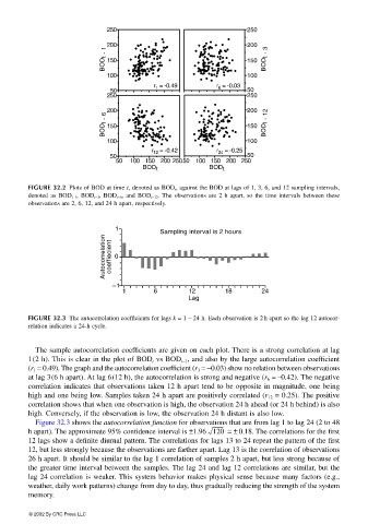
FIGURE 32.2 Plots of BOD at time t, denoted as BOD t , against the BOD at lags of 1, 3, 6, and 12 sampling intervals,
denoted as BOD t–1 , BOD t−3 , BOD t−6 , and BOD t−12 . The observations are 2 h apart, so the time intervals between these
observations are 2, 6, 12, and 24 h apart, respectively.

1
Sampling interval is 2 hours
Autocorrelation coeffiecient 0

–1
1 6 12 18 24
Lag

FIGURE 32.3 The autocorrelation coefficients for lags k = 1 − 24 h. Each observation is 2 h apart so the lag 12 autocor-
relation indicates a 24-h cycle.

The sample autocorrelation coefficients are given on each plot. There is a strong correlation at lag
1(2 h). This is clear in the plot of BOD t vs BOD t−1 , and also by the large autocorrelation coefficient
(r 1 = 0.49). The graph and the autocorrelation coefficient (r 3 = −0.03) show no relation between observations
at lag 3(6 h apart). At lag 6(12 h), the autocorrelation is strong and negative (r 6 = −0.42). The negative
correlation indicates that observations taken 12 h apart tend to be opposite in magnitude, one being
high and one being low. Samples taken 24 h apart are positively correlated (r 12 = 0.25). The positive
correlation shows that when one observation is high, the observation 24 h ahead (or 24 h behind) is also
high. Conversely, if the observation is low, the observation 24 h distant is also low.
Figure 32.3 shows the autocorrelation function for observations that are from lag 1 to lag 24 (2 to 48
h apart). The approximate 95% confidence interval is ±1.96 120 = ± 0.18. The correlations for the first
12 lags show a definite diurnal pattern. The correlations for lags 13 to 24 repeat the pattern of the first
12, but less strongly because the observations are farther apart. Lag 13 is the correlation of observations
26 h apart. It should be similar to the lag 1 correlation of samples 2 h apart, but less strong because of
the greater time interval between the samples. The lag 24 and lag 12 correlations are similar, but the
lag 24 correlation is weaker. This system behavior makes physical sense because many factors (e.g.,
weather, daily work patterns) change from day to day, thus gradually reducing the strength of the system
memory.

© 2002 By CRC Press LLC