Page 85 - Statistics for Environmental Engineers

L1592_Frame_C09 Page 78 Tuesday, December 18, 2001 1:45 PM

Suppose that the final result of an experiment, y, is given by y = a + b, where a and b are measured
values. If a and b each have a systematic error of +1, it is clear that the systematic error in y is +2. If,
however, a and b each have a random error between zero and ±1, the random error in y is not ±2. This
is because there will be occasions when the random error in a is positive and the error in b is negative
(or vice versa). The average random error in the true value will be zero if the measurements and
calculations are done many times. This means that the expected random error in y is zero. The variance
and standard deviation of the error in y will not be zero, but simple mathematical rules can be used to
estimate the precision of the final result if the precision of each observation (measurement) is known.
The rules for propagation of errors are explained in Chapters 10 and 49.
Repeated (replicate) measurements provide the means to quantify the measurement errors and
evaluate their importance. The effect of random errors can be reduced by averaging repeated measure-
ments. The error that remains can be quantified and statistical statements can be made about the
precision of the final results. Precision has to do with the scatter between replicate measurements.
Precise results have small random errors. The scatter caused by random errors cannot be eliminated
but it can minimized by careful technique. More importantly, it can be averaged and quantified.
The purpose of this chapter is to understand the statistical nature of experimental errors in the
laboratory. This was discussed briefly in Chapter 2 and will be discussed more in Chapters 10, 11, and
12. The APHA (1998) and ASTM (1990, 1992, 1993) provide detailed guidance on this subject.

Quantifying Precision

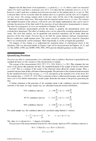
Precision can refer to a measurement or to a calculated value (a statistic). Precision is quantified by the
standard deviation (or the variance) of the measurement or statistic.
The average of five measurements [38.2, 39.7, 37.1, 39.0, 38.6] is = 38.5. This estimates the true
y
mean of the process that generates the data. The standard deviation of the sample of the five observations
is s = 0.97. This is a measure of the scatter of the observed values about the sample average. Thus, s
quantifies the precision of this collection of measurements. The precision of the estimated mean measured
= s/ n , also known as the standard error of the mean. For
by the standard deviation of the average, s y
5 = 0.43. This is a measure of how a collection of averages, each calculated
this example data, = 0.97/s y
from a set of five similar observations, would scatter about the true mean of the process generating the
data.
A further statement of the precision of the estimated mean is the confidence interval. Confidence
intervals of the mean, for large sample size, are calculated using the normal distribution:
σ σ
95% confidence interval y 1.96------- <– η < y + 1.96-------
n n
σ σ
99.7% confidence interval y 2.33------- <– η < y + 2.33-------
n n
σ σ
99% confidence interval y 2.58------- <– η < y + 2.58-------
n n

For small sample size, the confidence interval is calculated using Student’s t-statistic:
s
s
yt------- < η < y + t------- or yts y <– η < y + ts y
–
n n
The value of t is chosen for n − 1 degrees of freedom.
The precision of the mean estimated from the five observations, stated as a 95% confidence interval, is:
38.5 2.78 0.43) < η < 38.5 + 2.78 0.43)
(
(
–
37.3 << 39.7
n
© 2002 By CRC Press LLC