Page 87 - Statistics for Environmental Engineers

L1592_Frame_C09 Page 80 Tuesday, December 18, 2001 1:45 PM

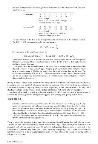
was kept blind to the fact that these specimens were not run-of-the-laboratory work. The mea-
sured values are:

Laboratory A 2.8 3.5 2.3 2.7 2.3 3.1 2.5
2.5 2.5 2.7 2.5 2.5 2.6 2.7
= 2.66 µg/L
y A
− C S = 2.66 − 2.50 = 0.16 µg/L
Bias = y A
Standard deviation = 0.32 µg/L
Laboratory B 5.3 4.7 3.6 5.0 3.6 4.5 4.6
4.3 3.9 4.1 4.2 4.2 4.3 4.9
= 4.38 µg/L
y B
– C S = 4.38 − 2.5 = 1.88 µg/L
Bias = y B
Standard deviation = 0.50 µg/L
The best estimate of the bias is the average minus the concentration of the standard solution.
The 100(1 − α)% confidence limits for the true bias are:
s
( yC S ) ± t ν=n−1,α/2 -------
–
n
For Laboratory A, the confidence interval is:
(
0.16 ± 2.160 0.32 14) = 0.16 ± 0.18 = – 0.03 to 0.34 µg/L
This interval includes zero, so we conclude with 95% confidence that the true bias is not greater
than zero. Laboratory B has a confidence interval of 1.88 ± 0.29, or 1.58 to 2.16 µg/L. Clearly,
the bias is greater than zero.
The precision of the two laboratories is the same; there is no significant difference between
standard deviations of 0.32 and 0.50 µg/L. Roughly speaking, the ratios of the variances would
have to exceed a value of 3 before we would reject the hypothesis that they are the same. The
2
2
ratio in this example is 0.5 0.32 = 2.5 . The test statistic (the “roughly three”) is the F-statistic
and this test is called the F-test on the variances. It will be explained more in Chapter 24 when we
discuss analysis of variance.
Having a “blind” analyst make measurements on specimens with known concentrations is the only way
to identify bias. Any certified laboratory must invest a portion of its effort in doing such checks on
measurement accuracy. Preparing test specimens with precisely known concentrations is not easy. Such
standard solutions can be obtained from certified laboratories (U.S. EPA labs, for example).
Another quality check is to split a well-mixed sample and add a known quantity of analyte to one or
more of the resulting portions. Example 9.3 suggests how splitting and spiking would work.
Example 9.3

Consider that the measured values in Example 9.2 were obtained in the following way. A large
portion of a test solution with unknown concentration was divided into 28 portions. To 14 of the
portions a quantity of analyte was added to increase the concentration by exactly 1.8 µg/L. The
true concentration is not known for the spiked or the unspiked specimens, but the measured
values should differ by 1.8 µg/L. The observed difference between labs A and B is 4.38 − 2.66 =
1.72 µg/L. This agrees with the true difference of 1.8 µg/L. This is presumptive evidence that
the two laboratories are doing good work.

There is a possible weakness in this kind of a comparison. It could happen that both labs are biased.
Suppose the true concentration of the master solution was 1 µg/L. Then, although the difference is as
expected, both labs are measuring about 1.5 µg/L too high, perhaps because there is some fault in the
measurement procedure they were given. Thus, “splitting and spiking” checks work only when one
laboratory is known to have excellent precision and low bias. This is the reason for having certified
reference laboratories.

© 2002 By CRC Press LLC