Page 81 - Sustainability in the Process Industry Integration and Optimization

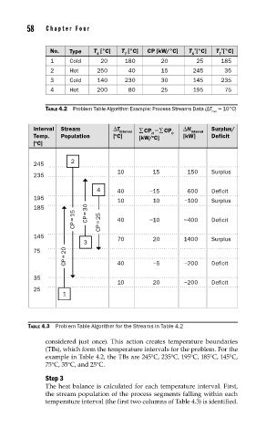
58 Cha p te r F o u r

*
No. Type T [°C] T [°C] CP [kW/°C] T [°C] T [°C]
*
T
S
T
S
1 Cold 20 180 20 25 185
2 Hot 250 40 15 245 35
3 Cold 140 230 30 145 235
4 Hot 200 80 25 195 75
TABLE 4.2 Problem Table Algorithm Example: Process Streams Data (ΔT = 10°C)
min

Interval Stream ∆T interval ∑ CP − ∑ CP ∆H interval Surplus/
H
o
Temp. Population [ C] [kW/ C] C [kW] Deficit
o
[ C]
o
245 2
10 15 150 Surplus
235
4 40 −15 600 Deficit
195 10 10 −100 Surplus
185
CP = 15 CP = 30 CP = 25 40 −10 −400 Deficit

145 70 20 1400 Surplus
3
CP = 20 CP = 20 40 −5 −200 Deficit
75

35
10 20 −200 Deficit
25
1

TABLE 4.3 Problem Table Algorithm for the Streams in Table 4.2

considered just once). This action creates temperature boundaries
(TBs), which form the temperature intervals for the problem. For the
example in Table 4.2, the TBs are 245°C, 235°C, 195°C, 185°C, 145°C,
75°C, 35°C, and 25°C.
Step 3
The heat balance is calculated for each temperature interval. First,
the stream population of the process segments falling within each
temperature interval (the first two columns of Table 4.3) is identified.