Page 82 - Sustainability in the Process Industry Integration and Optimization

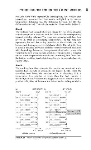
P r o c e s s I n t e g r a t i o n f o r I m p r ov i n g E n e r g y E f f i c i e n c y 59

Next, the sums of the segment CPs (heat capacity flow rates) in each
interval are calculated; then that sum is multiplied by the interval
temperature difference (i.e., the difference between the TBs that
define each interval). This calculation is also illustrated in Table 4.3.

Step 4
The Problem Heat Cascade shown in Figure 4.14 has a box allocated
to each temperature interval; each box contains the corresponding
interval enthalpy balances. The boxes are connected with heat flow
arrows in order of descending temperature. The top heat flow
represents the total hot utility provided to the cascade, and the
bottom heat flow represents the total cold utility. The hot utility flow
is initially assumed to be zero and this value is combined (summed)
with the enthalpy balance of the top cascade interval to produce the
value for the next lower cascade heat flow. This operation is repeated
for the lower temperature intervals and connecting heat flows until
the bottom heat flow is calculated, resulting in the cascade shown in
Figure 4.14(a).
Step 5
The resulting heat flow values in the cascade are examined, and a
feasible heat cascade is obtained; see Figure 4.14(b). From the
cascading heat flows, the smallest value is identified; if it is
nonnegative (i.e., positive or zero), then the heat cascade is
thermodynamically feasible. If a negative value is obtained then a
positive utility flow of the same absolute value has to be provided at

(a) HOT UTILITY (b) HOT UTILITY
245 °C 0 kW 245 °C 750 kW
ΔH = 150 kW ΔH = 150 kW
235 °C 150 kW 235 °C 900 kW
ΔH = −600 kW ΔH = −600 kW
195 °C −450 kW 195 °C 300 kW
ΔH = 100 kW ΔH = 100 kW
185 °C −350 kW 185 °C 400 kW
ΔH = −400 kW ΔH = −400 kW T HOT PINCH = 150°C
*
145 °C −750 kW 145 °C T PINCH 0 kW
T COLD PINCH = 140°C
ΔH = 1400 kW ΔH = 1400 kW
75 °C −650 kW 75 °C 1400 kW
ΔH = −200 kW ΔH = −200 kW
35 °C −450 kW 35 °C 1200 kW
ΔH = −200 kW ΔH = −200 kW
25 °C 250 kW 25 °C 1000 kW
HOT UTILITY HOT UTILITY
(a) Initial cascade (b) Feasible cascade
FIGURE 4.14 Heat Cascade for the process data in Table 4.2.