Page 86 - Sustainability in the Process Industry Integration and Optimization

P r o c e s s I n t e g r a t i o n f o r I m p r ov i n g E n e r g y E f f i c i e n c y 63

Construction of the Grand Composite Curve
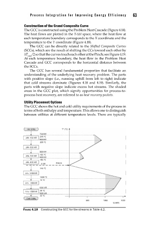
The GCC is constructed using the Problem Heat Cascade (Figure 4.14).
The heat flows are plotted in the T-ΔH space, where the heat flow at
each temperature boundary corresponds to the X coordinate and the
temperature to the Y coordinate (Figure 4.18).
The GCC can be directly related to the Shifted Composite Curves
(SCCs), which are the result of shifting the CCs toward each other by
ΔT /2 so that the curves touch each other at the Pinch; see Figure 4.19.
min
At each temperature boundary, the heat flow in the Problem Heat
Cascade and GCC corresponds to the horizontal distance between
the SCCs.
The GCC has several fundamental properties that facilitate an
understanding of the underlying heat recovery problem. The parts
with positive slope (i.e., running uphill from left to right) indicate
that cold streams dominate (Figures 4.18 and 4.19). Similarly, the
parts with negative slope indicate excess hot streams. The shaded
areas in the GCC plot, which signify opportunities for process-to-
process heat recovery, are referred to as heat recovery pockets.

Utility Placement Options
The GCC shows the hot and cold utility requirements of the process in
terms of both enthalpy and temperature. This allows one to distinguish
between utilities at different temperature levels. There are typically

Hot Utility T* (°C)
750 kW
245 °C
ΔH= 150 kW
900 kW
235 °C
ΔH= 600 kW
300 kW
195 °C
ΔH= 100 kW
400 kW
185 °C
ΔH= 400 kW
0 kW PINCH
145 °C
ΔH= 1400 kW
1400 °C
75 °C
ΔH= −200 kW
1200 kW
35 °C
ΔH= −200 kW
1000 kW
25 °C
Cold Utility
500 1000 1500
Q (kW)
FIGURE 4.18 Constructing the GCC for the streams in Table 4.2.