Page 88 - Sustainability in the Process Industry Integration and Optimization

P r o c e s s I n t e g r a t i o n f o r I m p r ov i n g E n e r g y E f f i c i e n c y 65

Higher complexity has several negative consequences, including
increased capital costs, greater potential for leaks, reduced safety,
and more maintenance expenses. Therefore limits are typically
placed on the number of steam levels.
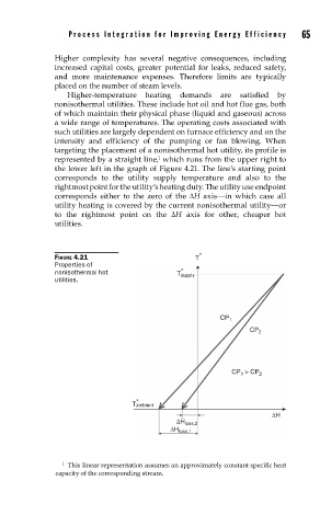
Higher-temperature heating demands are satisfied by
nonisothermal utilities. These include hot oil and hot flue gas, both
of which maintain their physical phase (liquid and gaseous) across
a wide range of temperatures. The operating costs associated with
such utilities are largely dependent on furnace efficiency and on the
intensity and efficiency of the pumping or fan blowing. When
targeting the placement of a nonisothermal hot utility, its profile is
1
represented by a straight line, which runs from the upper right to
the lower left in the graph of Figure 4.21. The line’s starting point
corresponds to the utility supply temperature and also to the
rightmost point for the utility’s heating duty. The utility use endpoint
corresponds either to the zero of the ΔH axis—in which case all
utility heating is covered by the current nonisothermal utility—or
to the rightmost point on the ΔH axis for other, cheaper hot
utilities.

FIGURE 4.21 T *
Properties of
nonisothermal hot T supply
*
utilities.

CP 1
CP 2

CP > CP 2
1

*
Tambient
ΔH
ΔH loss,2
ΔH loss,1

1 This linear representation assumes an approximately constant specifi c heat
capacity of the corresponding stream.