Page 180 - The Handbook for Quality Management a Complete Guide to Operational Excellence

166 P r o c e s s C o n t r o l Q u a n t i f y i n g P r o c e s s Va r i a t i o n 167

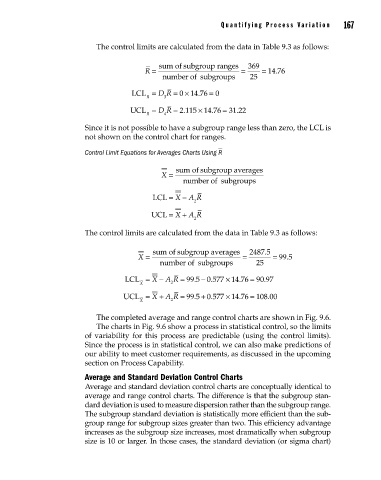
The control limits are calculated from the data in Table 9.3 as follows:

sum of subgroup ranges 369
R = = = 14 76
.
number of subgroups s 25
LCL = D R = × 14 76 = 0
0
.
R 3
.
UCL = D R = 2.1115 14 76× . = 31 22
R 4
Since it is not possible to have a subgroup range less than zero, the LCL is
not shown on the control chart for ranges.
Control Limit Equations for Averages Charts Using R

sum of subgroup averages
X =
number of subgroups
u
LCL = X − A R
2
UCL = X + A R
2
The control limits are calculated from the data in Table 9.3 as follows:

sum of subgroup averages 2487 5 .
X = = = 99 5 .
u
number of subgroups 25
×
.
LCL = X − A R = 99 5 0 577 14.776 = 90 97
.
− .
X 2
UCL = X + A R = 99 5 0 577 14 76 = 108 00
+
.
.
.
.
×
X 2
The completed average and range control charts are shown in Fig. 9.6.
The charts in Fig. 9.6 show a process in statistical control, so the limits
of variability for this process are predictable (using the control limits).
Since the process is in statistical control, we can also make predictions of
our ability to meet customer requirements, as discussed in the upcoming
section on Process Capability.
Average and Standard Deviation Control Charts
Average and standard deviation control charts are conceptually identical to
average and range control charts. The difference is that the subgroup stan-
dard deviation is used to measure dispersion rather than the subgroup range.
The subgroup standard deviation is statistically more efficient than the sub-
group range for subgroup sizes greater than two. This efficiency advantage
increases as the subgroup size increases, most dramatically when subgroup
size is 10 or larger. In those cases, the standard deviation (or sigma chart)

09_Pyzdek_Ch09_p151-208.indd 167 11/21/12 1:42 AM