Page 714 - The Mechatronics Handbook

0066_Frame_C23 Page 22 Wednesday, January 9, 2002 1:53 PM

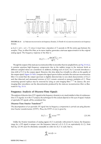
FIGURE 23.14 (a) Staircase reconstruction in frequency domain, (b) Result of staircase reconstruction in frequency
domain.

as h o (t) = u(t) − u(t − T s ) since it must have a duration of T s seconds to fill the entire gap between the
samples. Thus, in effect this filter, as its name implies, generates a staircase approximation to the original
analog signal. The frequency response of the filter is

sin ( πfT s ) – jπfT
H o f() = T ------------------------e s
πfT s
Though the output of the staircase reconstruction filter is smoother than its sampled form, see Fig. 23.14(a),
it contains spurious high-frequency components due to the sudden jumps in the staircase levels as
different sampled values are considered. In addition, holding each of x(nT s ) by T s seconds introduces a
time shift of T s /2 to the output signal. However, this time delay has virtually no effect on the quality of
the output signal. Figure 23.14(b) compares the signal spectra before and after the staircase reconstruction
filter. It is noted that the output spectrum is slightly distorted due to non-ideal characteristics of H o (f )
and that distorted and attenuated versions of X(f ) remain centered at nonzero multiples of F s . These
remaining spectral replicas may be removed by using an anti-imaging filter. 8,11,12 In essence, the anti-
imaging filter smoothens out the discontinuities produced by the staircase reconstruction filter as illus-
trated in Fig. 23.15.

Frequency Analysis of Discrete-Time Signals
The analysis of discrete-time (DT) signals in the frequency domain is very much similar to that of continuous-
time (CT) signals. As in the CT analysis, the techniques for the analysis depend on the type of signal. Analysis
of aperiodic DT signals will be considered first.

Discrete-Time Fourier Transform 6–8
The decomposition of an aperiodic DT signal into its frequency components is carried out using discrete-
time Fourier transformation (DTFT). Thus, the DTFT of x(n) is given by

∞
Xf() = ∑ xn()e – j2πfn (23.39)
n=∞
–
Unlike the Fourier transform of analog signal, X( f ) is periodic with period F s ; hence, the frequency
range for a DT signal is unique over the frequency interval (−F s /2, F s /2) or, equivalently (0, F s ). Note
that Eq. (23.39) must be absolutely summable in order for X( f ) to exist, that is,

∞
∑ xn() < ∞
n=∞
–

©2002 CRC Press LLC