Page 719 - The Mechatronics Handbook

0066_Frame_C23 Page 27 Wednesday, January 9, 2002 1:53 PM

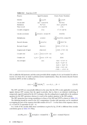
TABLE 23.9 Properties of DFT
Property Signal Description Discrete Fourier Transform
Q Q
Linearity ∑ a m x m n() ∑ a m X m k()
m=0 m=0
(
[
km
Circular shift xn – m)mod N] W N Xk()
(
[
qn
–
Modulation W N xn() Xk – q)mod N]
∗ ∗
[
Time reversal x – n mod N] x k()
∗
∗
[
Complex conjugation x n() X – k mod N]
N−1
[
(
Circular convolution ∑ xm()yn – m)mod N] X k() Y k()
m=0
N−1
1
(
[
y
Multiplication x n() n() ---- ∑ Xm()Yk – m)mod N]
N
m=0
N−1 1 N−1
∗
∗
Parseval’s theorem ∑ xn()y n() ---- ∑ Xk()Y k()
N
k=0 k=0
{
∗
Real part of signal Re xn()} 1 -- Xk() +{ X N –( k)}
2
{
(
∗
Imaginary part of signal j Im xn()} 1 -- Xk() –{ X N – k)}
2
∗
Complex even x ce n() = 1 -- xn() +{ x N –( n)} X R k()
2
∗
Complex odd x co n() = 1 -- xn() –{ x N –( n)} jX I k()
2
∗
(
Any real signal xn() Xk() = X N – k)
X R k() = X R N – k)
(
(
X I k() = – X I N – k)
Xk() = XN – k)
(
∠ Xk() = – ∠ XN – k)
(
X(k) is called the kth harmonic and this exists provided all the samples of x(n) are bounded. In order to
recover x(n) from X(k) we need to perform inverse transformation. Thus, the inverse discrete Fourier
transform (IDFT) of X(k) is defined as
N−1
1
xn() = ---- ∑ Xk()W N , n = 0,1,…,N 1 (23.47)
kn
–
–
N
k=0
The DFT and DFS are conceptually different in the sense that the DFS is only applicable to periodic
signals whereas DFT assumes that the signal is periodic, that is, there is an inherent windowing of
nonperiodic signal if analyzed by the DFT technique. Also the scaling factor is applicable to the synthesis
equation for the DFT operation, whereas it is used in the analysis equation in the DFS analysis.
The DFT properties bear strong resemblance to those of the DFS and DTFT as shown in Table 23.9.
The following should be noted in the DFT computation: Circular shift operation can be considered
as wrapping the part of the sequence that falls outside of 0 to N − 1 to the front of the sequence, that is,
x[(−n) mod N] is equivalent to x(N − n).
As a result of the circular shift, linear convolution as given by Eq. (23.40) is different from circular
convolution given in Table 23.9. Thus,
N−1 N−1
(
xn()⊗ N yn() = ∑ xm()yn m)mod N] = ∑ xn m)mod N]ym()
[
(
[
–
–
m=0 m=0
©2002 CRC Press LLC